|
Probabilistic Co-Occurrence Report for Atrazine and 10 Endangered Species
|
 |
Table of Contents
- Pesticide Use Modeling
- Methods
- Results
- Atrazine Applications on Corn
- Species Distribution Modeling
- Methods
- Results
- Aphelocoma coerulescens
- Bombus affinis
- Bufo houstonensis
- Chamaesyce garberi
- Cicindela puritana
- Eurycea tonkawae
- Lycaeides melissa samuelis
- Neonympha mitchellii mitchellii
- Pedicularis furbishiae
- Tympanuchus cupido attwateri
- Co-Occurrence Modeling
- Methods
- Results
- Aphelocoma coerulescens and Atrazine Applications on Corn
- Bombus affinis and Atrazine Applications on Corn
- Bufo houstonensis and Atrazine Applications on Corn
- Chamaesyce garberi and Atrazine Applications on Corn
- Cicindela puritana and Atrazine Applications on Corn
- Eurycea tonkawae and Atrazine Applications on Corn
- Lycaeides melissa samuelis and Atrazine Applications on Corn
- Neonympha mitchellii mitchellii and Atrazine Applications on Corn
- Pedicularis furbishiae and Atrazine Applications on Corn
- Tympanuchus cupido attwateri and Atrazine Applications on Corn
- Summary
- References
|
Foreword
In response to the need for efficient production of advanced geospatial analyses of co-occurrence between pesticide use and species of interest as required by the Endangered Species Act, Stone Environmental, with the support of Syngenta Crop Protection, developed the Automated Probabilistic Co-Occurrence Assessment Tool (APCOAT)[1] in early 2022. APCOAT is designed to produce probabilistic spatial models of both pesticide use and species distributions, and combine the models for co-occurrence assessments. Each of the models may also be run independently. The pesticide use models are represented by probabilistic crop footprints[2] and statistical measures of the Percent Crop Treated (PCT) derived from freely available pesticide usage data[3], or from pesticide usage data provided by the user. The species distribution models (SDMs) are produced using maximum entropy methods[4] analyzing the statistical fit between species presence location records and geographic predictor rasters for environmental variables[5]. Probabilistic co-occurrence between pesticide usage and species distributions is calculated by multiplying the two model output rasters. For planning and conservation purposes, the co-occurrence statistics may be summarized by state, crop reporting district, county, or watershed.
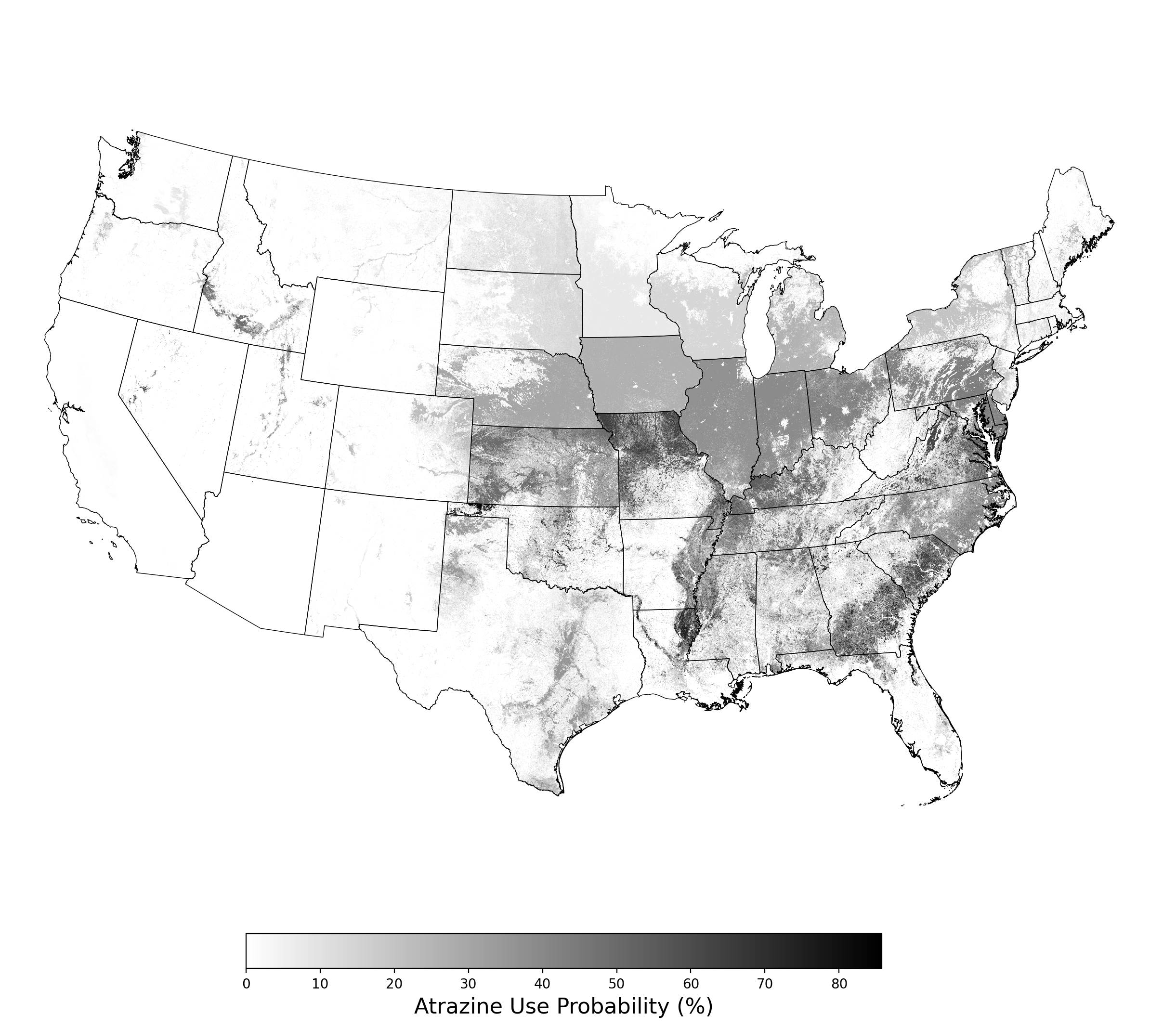
This case study is a compilation of co-occurrence reports between atrazine use on corn and 10 endangered species, generated in February 2022 using APCOAT. In these assessments the probabilistic pesticide use estimates are represented by probabilistic crop footprints and estimates atrazine use on corn for years 2012 - 2017 at the state level. Probabilities of crop presence are calculated at 30m resolution based on the fraction of years the crop is present from 2015 - 2020 in the Cropland Data Layer (CDL)[6], and adjusted by estimates of crop mapping accuracy[7] and crop production[8] using Bayesian inference. The PCT statistics applied to the probabilistic crop footprints assume that atrazine is applied at the maximum permitted rate of 2 lb/ac per year[9]. Probabilistic species distribution models are produced based on the statistical fit between species presence records and geographic environmental predictor variable datasets: monthly solar radiation[10], bioclimatic variables derived from precipitation and temperature[10], elevation[10], and land use/land cover[11]. Co-occurrence between probabilistic pesticide use and probabilistic species distributions is calculated by multiplying the probabilistic pesticide use footprint by the probabilistic species distribution model, and is summarized at the HUC8 scale.
|
1. Pesticide Use Modeling From ePest
1.1 Pesticide Use Modeling Methods
APCOAT pesticide use footprints are generated by first using pesticide use and crop acreage data to create region-specific rasters of the percent crop treated (PCT) for the pesticide of interest. The PCT rasters are then multiplied by probabilistic crop footprint rasters[2] that are included in the software package. The PCT rasters are created by first calculating an annual time series of the maximum potential annual usage in a region. Maximum annual usage is calculated by multiplying the regional crop acreage measured from CDL for 2012 - 2017 years by the specified application rates (Table 1). Regional pesticide usage data is then divided by the maximum potential usage in each year to generate an annual PCT time series for each region. Finally, a user-specified statistic is calculated from these regional time series' and converted to raster format.
Table 1. Modeling parameters for calculations of probabilistic usage of atrazine.
| Crop |
corn
|
| Application rate (lb/ac) |
2.50 |
| Data source |
ePest |
| Data source resolution |
state |
| Summary statistic |
maximum |
1.2 Pesticide Use Modeling Results
The pesticide use modeling results consists of the following figure and table for each crop modeled:
- A map of the probabilistic use footprint produced by multiplying the PCT raster by the probabilistic crop footprint (Figure 1)
- A table showing a range of statistics for the annual PCT time series calculated for each region, as well as the statistic selected for the analysis (maximum) (Table 1)
1.3 Pesticide Use Modeling Results for Corn.
| State |
State_FIPS |
Minimum |
10th Percentile |
25th Percentile |
Median |
75th Percentile |
90th Percentile |
Maximum |
Selected Statistic: Maximum |
| Alabama |
1 |
41.8% |
41.8% |
54.3% |
54.7% |
55.6% |
62.1% |
62.1% |
62.1% |
| Arizona |
4 |
0.0% |
0.0% |
0.0% |
0.0% |
0.0% |
0.1% |
0.1% |
0.1% |
| Arkansas |
5 |
46.4% |
46.6% |
47.2% |
58.1% |
61.5% |
68.6% |
68.6% |
68.6% |
| California |
6 |
0.8% |
0.8% |
1.1% |
1.2% |
1.4% |
1.6% |
1.6% |
1.6% |
| Colorado |
8 |
11.6% |
14.1% |
18.4% |
19.7% |
22.3% |
23.8% |
24.1% |
24.1% |
| Connecticut |
9 |
0.8% |
0.8% |
8.3% |
10.7% |
15.1% |
19.1% |
19.1% |
19.1% |
| Delaware |
10 |
17.9% |
17.9% |
26.0% |
38.6% |
43.7% |
50.6% |
50.6% |
50.6% |
| Florida |
12 |
21.1% |
21.1% |
29.0% |
37.8% |
66.2% |
68.1% |
68.1% |
68.1% |
| Georgia |
13 |
55.2% |
55.2% |
65.8% |
67.6% |
71.4% |
86.0% |
90.2% |
90.2% |
| Idaho |
16 |
0.0% |
0.0% |
1.9% |
2.1% |
3.7% |
17.9% |
55.9% |
55.9% |
| Illinois |
17 |
34.2% |
34.2% |
34.3% |
34.8% |
36.9% |
37.0% |
37.0% |
37.0% |
| Indiana |
18 |
30.3% |
30.3% |
31.2% |
34.5% |
37.3% |
39.9% |
39.9% |
39.9% |
| Iowa |
19 |
20.6% |
20.6% |
20.7% |
23.2% |
26.4% |
26.6% |
26.6% |
26.6% |
| Kansas |
20 |
37.8% |
37.8% |
40.4% |
44.7% |
47.9% |
49.4% |
49.4% |
49.4% |
| Kentucky |
21 |
31.8% |
31.8% |
37.2% |
43.2% |
44.7% |
53.8% |
54.3% |
54.3% |
| Louisiana |
22 |
52.7% |
52.7% |
61.8% |
72.0% |
79.9% |
80.1% |
80.1% |
80.1% |
| Maine |
23 |
7.6% |
7.6% |
17.7% |
21.6% |
25.0% |
25.5% |
25.5% |
25.5% |
| Maryland |
24 |
27.1% |
27.1% |
36.1% |
43.9% |
47.0% |
47.3% |
47.8% |
47.8% |
| Massachusetts |
25 |
4.2% |
4.2% |
5.8% |
8.6% |
10.6% |
19.8% |
19.8% |
19.8% |
| Michigan |
26 |
16.4% |
16.5% |
18.6% |
19.5% |
20.0% |
28.6% |
28.6% |
28.6% |
| Minnesota |
27 |
3.1% |
3.1% |
3.4% |
5.2% |
7.1% |
7.6% |
7.6% |
7.6% |
| Mississippi |
28 |
15.9% |
15.9% |
40.9% |
44.3% |
57.3% |
68.1% |
68.1% |
68.1% |
| Missouri |
29 |
48.7% |
48.7% |
51.6% |
59.3% |
60.6% |
64.1% |
64.1% |
64.1% |
| Montana |
30 |
3.5% |
3.5% |
5.4% |
12.0% |
14.0% |
17.6% |
17.7% |
17.7% |
| Nebraska |
31 |
21.5% |
21.5% |
23.4% |
26.4% |
30.5% |
30.7% |
30.7% |
30.7% |
| Nevada |
32 |
2.3% |
2.4% |
3.2% |
43.3% |
100.0% |
100.0% |
100.0% |
100.0% |
| New Hampshire |
33 |
8.3% |
8.3% |
8.3% |
10.5% |
15.8% |
19.6% |
19.6% |
19.6% |
| New Jersey |
34 |
9.7% |
9.7% |
17.6% |
20.1% |
27.0% |
27.5% |
27.5% |
27.5% |
| New Mexico |
35 |
1.9% |
3.0% |
4.5% |
7.8% |
17.0% |
17.7% |
17.8% |
17.8% |
| New York |
36 |
15.4% |
16.0% |
16.4% |
18.3% |
20.2% |
24.1% |
24.1% |
24.1% |
| North Carolina |
37 |
28.0% |
28.5% |
33.8% |
42.0% |
51.4% |
53.9% |
54.3% |
54.3% |
| North Dakota |
38 |
4.7% |
5.9% |
8.6% |
9.4% |
13.1% |
13.7% |
14.7% |
14.7% |
| Ohio |
39 |
34.7% |
34.7% |
36.7% |
39.7% |
41.7% |
42.4% |
42.4% |
42.4% |
| Oklahoma |
40 |
31.3% |
38.0% |
42.3% |
56.9% |
84.1% |
84.7% |
85.8% |
85.8% |
| Oregon |
41 |
1.3% |
1.4% |
2.6% |
6.9% |
17.7% |
32.5% |
33.6% |
33.6% |
| Pennsylvania |
42 |
28.4% |
28.5% |
29.0% |
29.6% |
42.8% |
46.4% |
46.4% |
46.4% |
| Rhode Island |
44 |
3.8% |
3.8% |
6.2% |
7.5% |
8.1% |
11.1% |
11.1% |
11.1% |
| South Carolina |
45 |
39.6% |
39.6% |
44.5% |
61.2% |
61.7% |
75.6% |
75.6% |
75.6% |
| South Dakota |
46 |
10.0% |
10.3% |
11.0% |
11.5% |
12.8% |
15.1% |
15.2% |
15.2% |
| Tennessee |
47 |
30.1% |
30.1% |
32.1% |
43.6% |
47.1% |
54.3% |
54.3% |
54.3% |
| Texas |
48 |
23.2% |
23.6% |
25.6% |
30.9% |
32.4% |
34.4% |
35.6% |
35.6% |
| Utah |
49 |
4.2% |
4.5% |
4.7% |
9.3% |
20.0% |
34.6% |
41.2% |
41.2% |
| Vermont |
50 |
8.1% |
8.1% |
8.8% |
17.2% |
23.4% |
30.6% |
30.6% |
30.6% |
| Virginia |
51 |
33.1% |
33.1% |
43.1% |
44.8% |
60.6% |
68.9% |
68.9% |
68.9% |
| Washington |
53 |
0.8% |
1.2% |
1.5% |
4.7% |
6.8% |
13.4% |
14.8% |
14.8% |
| West Virginia |
54 |
12.3% |
12.3% |
24.6% |
27.1% |
34.6% |
37.1% |
37.1% |
37.1% |
| Wisconsin |
55 |
11.9% |
11.9% |
12.8% |
13.8% |
14.2% |
15.0% |
15.0% |
15.0% |
| Wyoming |
56 |
0.3% |
0.4% |
0.5% |
6.7% |
10.3% |
12.1% |
14.5% |
14.5% |
2. Species Distribution Modeling
2.1 Species Distribution Modeling Methods
APCOAT uses Maxent software[4] to compare species location records to environmental variables and locate areas of similar habitat suitability as the basis for generating Species Distribution Models. Specifically, Maxent uses presence-only species records to "minimize the relative entropy between two probability densities (one estimated from the presence data and one, from the landscape) defined in covariate space"[5] and generate probabilistic models. Since the probabilistic models vary slightly with each solution, APCOAT generates 5 models at a time and evaluates the average of the 5 models iteratively. Iterative evaluation of the averaged models follows a set of best practice methods to select the best-fit model that uses the fewest predictor variables and mizimizes correlation among these predictors[12]. Eighty percent of the species location records are used in the initial model training iterations, and the remaining twenty percent of species location records are used for evaluation of the final model. In this case study environmental conditions were modeled using solar radiation[10], bioclimatic (Table 3[10]), elevation [10], and land use/land cover data[11]. Species location data were provided by NatureServe[13].
Table 3. Reference table for WorldClim bioclimatic variables
Bioclim1 = Annual Mean Temperature
Bioclim2 = Mean Diurnal Range (Mean of monthly (max temp - min temp))
Bioclim3 = Isothermality ((BIO2/BIO7) x100)
Bioclim4 = Temperature Seasonality (standard deviation x100)
Bioclim5 = Max Temperature of Warmest Month
Bioclim6 = Min Temperature of Coldest Month
Bioclim7 = Temperature Annual Range (BIO5-BIO6)
Bioclim8 = Mean Temperature of Wettest Quarter
Bioclim9 = Mean Temperature of Driest Quarter
Bioclim10 = Mean Temperature of Warmest Quarter
Bioclim11 = Mean Temperature of Coldest Quarter
Bioclim12 = Annual Precipitation
Bioclim13 = Precipitation of Wettest Month
Bioclim14 = Precipitation of Driest Month
Bioclim15 = Precipitation Seasonality (Coefficient of Variation)
Bioclim16 = Precipitation of Wettest Quarter
Bioclim17 = Precipitation of Driest Quarter
Bioclim18 = Precipitation of Warmest Quarter
Bioclim19 = Precipitation of Coldest Quarter
|
2.2 Species Distribution Modeling Results
2.2.1 Aphelocoma coerulescens
2.2.2 Bombus affinis
2.2.3 Bufo houstonensis
2.2.4 Chamaesyce garberi
2.2.5 Cicindela puritana
2.2.6 Eurycea tonkawae
2.2.7 Lycaeides melissa samuelis
2.2.8 Neonympha mitchellii mitchellii
2.2.9 Pedicularis furbishiae
2.2.10 Tympanuchus cupido attwateri
2.2.1 Species Distribution Modeling - Aphelocoma coerulescens
The species distribution modeling results consist of the following figures and tables:
- A table showing the SDM inputs (Table 4)
- A map showing the extent of SDM coverage (Figure 2)
- A graph showing the correlation between the predictor variable selected for evaluation (Figure 3)
- A graph of the model fit of each SDM iteration as measured by total Area Under Curve (AUC) where the curve is the Receiver Operating Curve, based on training data (Figure 4)
- A table showing the diagnostic statistics of the training data used in the final selected SDM iteration (Table 5)
- Graphs illustrating the predictor variable values sampled by the species observations and randomly selected background locations for continuous variables (Figure 5), and discrete variables (Figure 6)
- A graph showing the percent contribution of each predictor variable to the final selected SDM (Figure 7)
- A table showing the mean AUC for each of the five model runs that are averaged for the final selected SDM (Table 6)
- A map of the final averaged SDM (Figure 8)
Table 4. Input parameters for species distribution modeling of Aphelocoma coerulescens.
| Number of predictors |
33 |
| Names of predictors |
Bioclim.01.tif, Bioclim.02.tif, Bioclim.03.tif, Bioclim.04.tif,
Bioclim.05.tif, Bioclim.06.tif, Bioclim.07.tif, Bioclim.08.tif,
Bioclim.09.tif, Bioclim.10.tif, Bioclim.11.tif, Bioclim.12.tif,
Bioclim.13.tif, Bioclim.14.tif, Bioclim.15.tif, Bioclim.16.tif,
Bioclim.17.tif, Bioclim.18.tif, Bioclim.19.tif, Elevation.tif,
Solar.APR.tif, Solar.AUG.tif, Solar.DEC.tif, Solar.FEB.tif,
Solar.JAN.tif, Solar.JUL.tif, Solar.JUN.tif, Solar.MAR.tif,
Solar.MAY.tif, Solar.NOV.tif, Solar.OCT.tif, Solar.SEP.tif,
USGS_LULC.tif |
| Predictor correlation threshold |
0.67 |
| Predictor contribution threshold |
1.0 |
| SDM threshold |
0.2 |
| Number of iterations conducted |
3 |
| Final SDM iteration number |
2 |
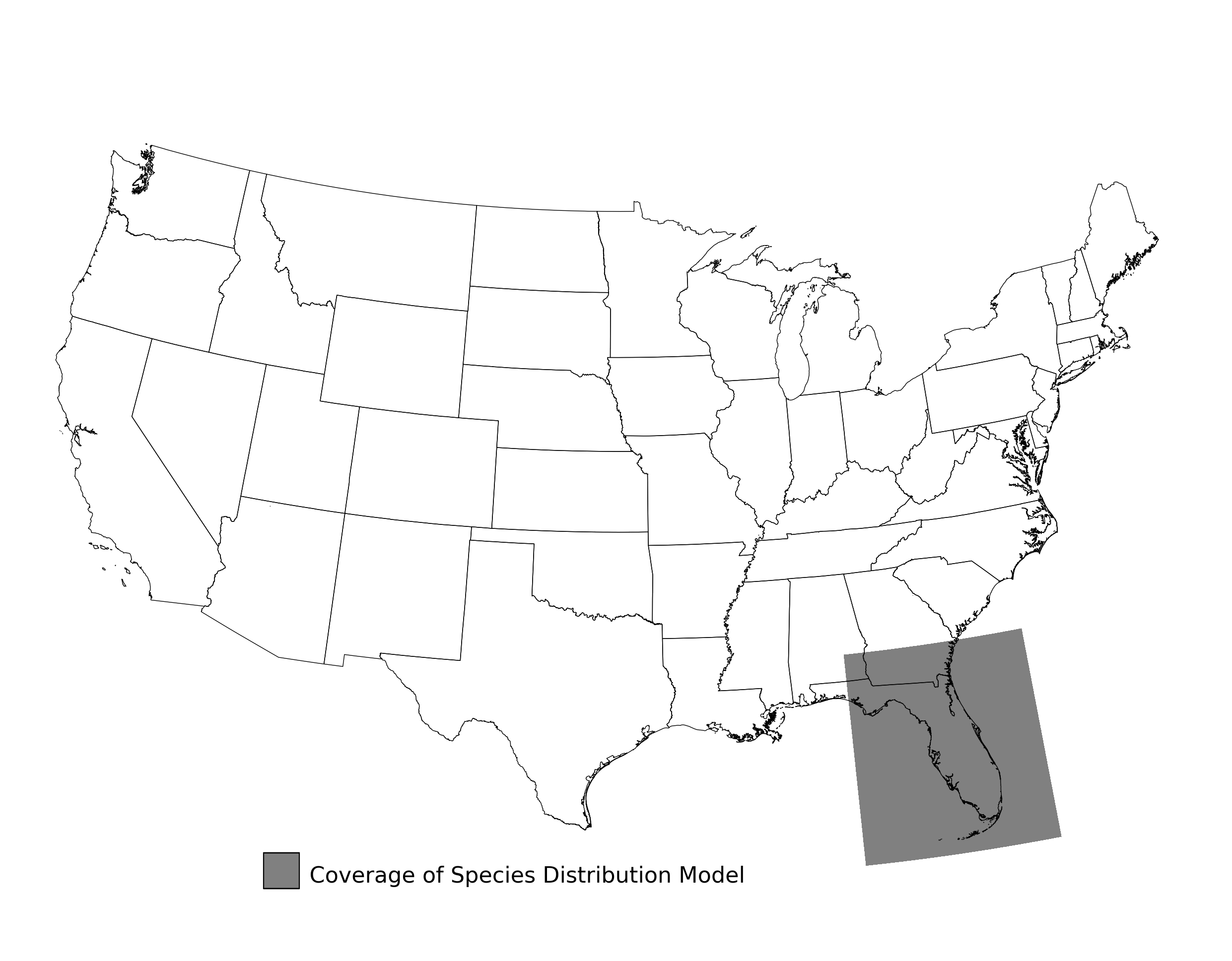
Figure 2. Extent of the species range modeled for Aphelocoma coerulescens. Modeling extent is determined by buffering species location records in all directions by 3 degrees latitude/longitude.
|
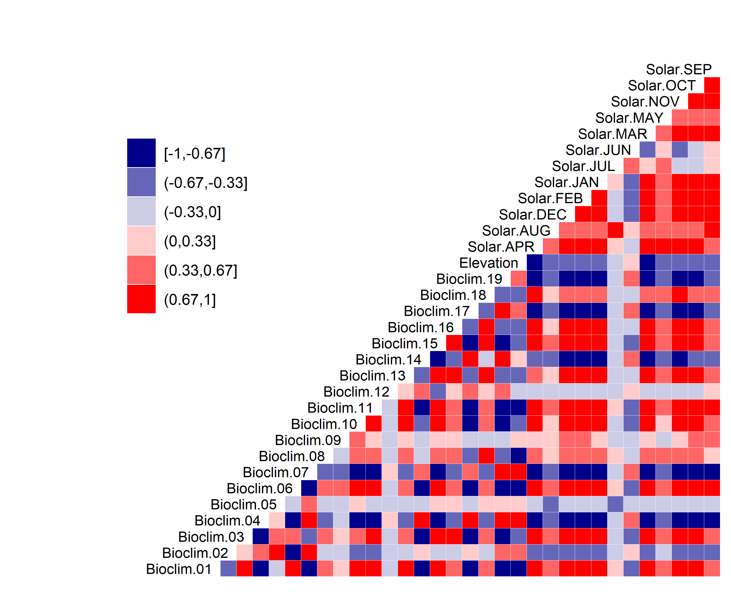
Figure 3. Correlation between SDM predictor variables for Aphelocoma coerulescens.
|
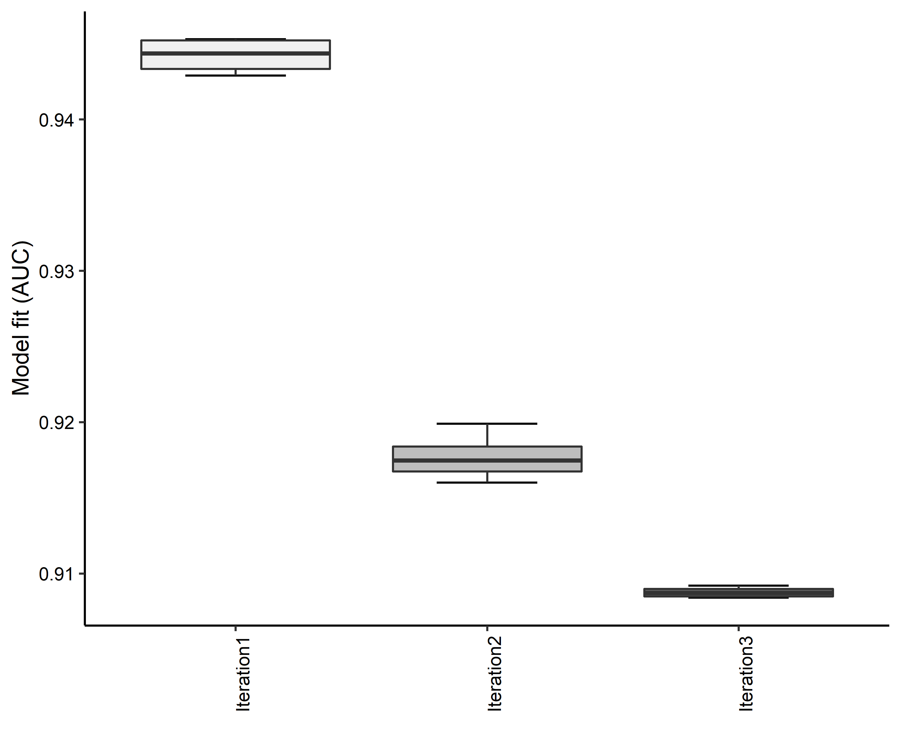
Figure 4. Boxplots of model fit for each iteration of Aphelocoma coerulescens distribution modeling. Statistics are calculated using 80% of species location records reserved for model training.
|
Table 5. Diagnostic statistics of the training data used in SDM iteration #2 for Aphelocoma coerulescens.
| Model Output |
Realization 1 |
Realization 2 |
Realization 3 |
Realization 4 |
Realization 5 |
Mean |
Standard Deviation |
| Number of training samples |
366.0000 |
366.0000 |
366.0000 |
366.0000 |
366.0000 |
366.00000 |
0.000000 |
| Regularized training gain |
1.3791 |
1.3543 |
1.3560 |
1.3420 |
1.3729 |
1.36086 |
0.015000 |
| Unregularized training gain |
1.5379 |
1.5178 |
1.5242 |
1.4934 |
1.5448 |
1.52362 |
0.020000 |
| Iterations |
500.0000 |
500.0000 |
500.0000 |
500.0000 |
500.0000 |
500.00000 |
0.000000 |
| Training AUC |
0.9201 |
0.9170 |
0.9179 |
0.9160 |
0.9199 |
0.91818 |
0.001794 |
| Number of background points |
10366.0000 |
10366.0000 |
10366.0000 |
10366.0000 |
10366.0000 |
10366.00000 |
0.000000 |
| Bioclim 04 contribution |
63.6355 |
60.6916 |
59.8011 |
62.1869 |
58.7740 |
61.01782 |
1.926172 |
| Bioclim 09 contribution |
7.8460 |
7.6063 |
9.0431 |
8.5832 |
9.6500 |
8.54572 |
0.842666 |
| Bioclim 18 contribution |
9.0072 |
10.0333 |
9.4937 |
9.6685 |
10.2729 |
9.69512 |
0.490588 |
| Elevation contribution |
2.3956 |
4.3426 |
6.9860 |
4.8445 |
6.6677 |
5.04728 |
1.867719 |
| Solar AUG contribution |
7.3713 |
6.8350 |
6.4292 |
6.1879 |
5.3225 |
6.42918 |
0.764074 |
| Solar MAY contribution |
3.5868 |
3.2547 |
2.2148 |
2.8420 |
2.8497 |
2.94960 |
0.514927 |
| USGS_LULC contribution |
6.1576 |
7.2365 |
6.0322 |
5.6870 |
6.4631 |
6.31528 |
0.585284 |
| Bioclim 04 permutation importance |
55.6743 |
56.7567 |
54.1867 |
58.2692 |
55.7245 |
56.12228 |
1.509730 |
| Bioclim 09 permutation importance |
10.6227 |
8.9739 |
9.9152 |
9.4705 |
11.0400 |
10.00446 |
0.838108 |
| Bioclim 18 permutation importance |
9.3591 |
10.5840 |
10.2554 |
9.2666 |
8.6269 |
9.61840 |
0.792500 |
| Elevation permutation importance |
4.5521 |
4.6590 |
5.6523 |
6.1083 |
6.5994 |
5.51422 |
0.895362 |
| Solar AUG permutation importance |
9.0185 |
9.5995 |
9.7463 |
9.0314 |
9.0723 |
9.29360 |
0.350683 |
| Solar MAY permutation importance |
8.2525 |
7.9646 |
8.6451 |
6.5616 |
7.0622 |
7.69720 |
0.861857 |
| USGS_LULC permutation importance |
2.5207 |
1.4623 |
1.5988 |
1.2925 |
1.8748 |
1.74982 |
0.480753 |
| Entropy |
7.8722 |
7.8953 |
7.8974 |
7.9091 |
7.8771 |
7.89022 |
0.015253 |
| Prevalence average probability of presence over background sites |
0.1486 |
0.1523 |
0.1528 |
0.1545 |
0.1495 |
0.15154 |
0.002436 |
| Fixed cumulative value 1 cumulative threshold |
1.0000 |
1.0000 |
1.0000 |
1.0000 |
1.0000 |
1.00000 |
0.000000 |
| Fixed cumulative value 1 Cloglog threshold |
0.0432 |
0.0458 |
0.0450 |
0.0439 |
0.0423 |
0.04404 |
0.001394 |
| Fixed cumulative value 1 area |
0.4233 |
0.4347 |
0.4289 |
0.4336 |
0.4272 |
0.42954 |
0.004689 |
| Fixed cumulative value 1 training omission |
0.0109 |
0.0109 |
0.0109 |
0.0109 |
0.0109 |
0.01090 |
0.000000 |
| Fixed cumulative value 5 cumulative threshold |
5.0000 |
5.0000 |
5.0000 |
5.0000 |
5.0000 |
5.00000 |
0.000000 |
| Fixed cumulative value 5 Cloglog threshold |
0.1398 |
0.1390 |
0.1445 |
0.1431 |
0.1391 |
0.14110 |
0.002533 |
| Fixed cumulative value 5 area |
0.3121 |
0.3217 |
0.3177 |
0.3211 |
0.3146 |
0.31744 |
0.004129 |
| Fixed cumulative value 5 training omission |
0.0219 |
0.0273 |
0.0246 |
0.0219 |
0.0219 |
0.02352 |
0.002415 |
| Fixed cumulative value 10 cumulative threshold |
10.0000 |
10.0000 |
10.0000 |
10.0000 |
10.0000 |
10.00000 |
0.000000 |
| Fixed cumulative value 10 Cloglog threshold |
0.2204 |
0.2197 |
0.2305 |
0.2274 |
0.2223 |
0.22406 |
0.004694 |
| Fixed cumulative value 10 area |
0.2473 |
0.2557 |
0.2543 |
0.2568 |
0.2501 |
0.25284 |
0.004006 |
| Fixed cumulative value 10 training omission |
0.0574 |
0.0546 |
0.0601 |
0.0574 |
0.0546 |
0.05682 |
0.002307 |
| Minimum training presence cumulative threshold |
0.4422 |
0.4600 |
0.4852 |
0.4354 |
0.3445 |
0.43346 |
0.053328 |
| Minimum training presence Cloglog threshold |
0.0184 |
0.0207 |
0.0205 |
0.0193 |
0.0146 |
0.01870 |
0.002475 |
| Minimum training presence area |
0.4693 |
0.4776 |
0.4706 |
0.4815 |
0.4864 |
0.47708 |
0.007232 |
| Minimum training presence training omission |
0.0000 |
0.0000 |
0.0000 |
0.0000 |
0.0000 |
0.00000 |
0.000000 |
| X10 percentile training presence cumulative threshold |
14.8925 |
14.0133 |
14.2228 |
14.4048 |
13.9952 |
14.30572 |
0.368421 |
| X10 percentile training presence Cloglog threshold |
0.2883 |
0.2754 |
0.2852 |
0.2864 |
0.2777 |
0.28260 |
0.005691 |
| X10 percentile training presence area |
0.2049 |
0.2191 |
0.2174 |
0.2178 |
0.2149 |
0.21482 |
0.005750 |
| X10 percentile training presence training omission |
0.0984 |
0.0984 |
0.0984 |
0.0984 |
0.0984 |
0.09840 |
0.000000 |
| Equal training sensitivity and specificity cumulative threshold |
22.3147 |
21.3585 |
21.9267 |
22.1846 |
22.2077 |
21.99844 |
0.385076 |
| Equal training sensitivity and specificity Cloglog threshold |
0.3743 |
0.3629 |
0.3697 |
0.3761 |
0.3736 |
0.37132 |
0.005255 |
| Equal training sensitivity and specificity area |
0.1585 |
0.1694 |
0.1667 |
0.1668 |
0.1617 |
0.16462 |
0.004413 |
| Equal training sensitivity and specificity training omission |
0.1585 |
0.1694 |
0.1667 |
0.1667 |
0.1612 |
0.16450 |
0.004488 |
| Maximum training sensitivity plus specificity cumulative threshold |
11.9250 |
11.6949 |
11.5643 |
12.4347 |
11.1152 |
11.74682 |
0.484737 |
| Maximum training sensitivity plus specificity Cloglog threshold |
0.2473 |
0.2430 |
0.2528 |
0.2605 |
0.2405 |
0.24882 |
0.008026 |
| Maximum training sensitivity plus specificity area |
0.2290 |
0.2391 |
0.2395 |
0.2339 |
0.2394 |
0.23618 |
0.004655 |
| Maximum training sensitivity plus specificity training omission |
0.0683 |
0.0628 |
0.0656 |
0.0738 |
0.0628 |
0.06666 |
0.004599 |
| Balance training omission predicted area and threshold value cumulative threshold |
2.3046 |
3.0250 |
2.2744 |
2.5288 |
2.1897 |
2.46450 |
0.337460 |
| Balance training omission predicted area and threshold value Cloglog threshold |
0.0815 |
0.0972 |
0.0813 |
0.0901 |
0.0770 |
0.08542 |
0.008123 |
| Balance training omission predicted area and threshold value area |
0.3706 |
0.3629 |
0.3774 |
0.3739 |
0.3769 |
0.37234 |
0.005937 |
| Balance training omission predicted area and threshold value training omission |
0.0109 |
0.0109 |
0.0109 |
0.0109 |
0.0109 |
0.01090 |
0.000000 |
| Equate entropy of thresholded and original distributions cumulative threshold |
9.4531 |
9.7024 |
9.4882 |
9.4583 |
9.5992 |
9.54024 |
0.108152 |
| Equate entropy of thresholded and original distributions Cloglog threshold |
0.2113 |
0.2153 |
0.2224 |
0.2195 |
0.2144 |
0.21658 |
0.004378 |
| Equate entropy of thresholded and original distributions area |
0.2530 |
0.2589 |
0.2595 |
0.2625 |
0.2543 |
0.25764 |
0.003916 |
| Equate entropy of thresholded and original distributions training omission |
0.0464 |
0.0519 |
0.0546 |
0.0574 |
0.0519 |
0.05244 |
0.004072 |
|
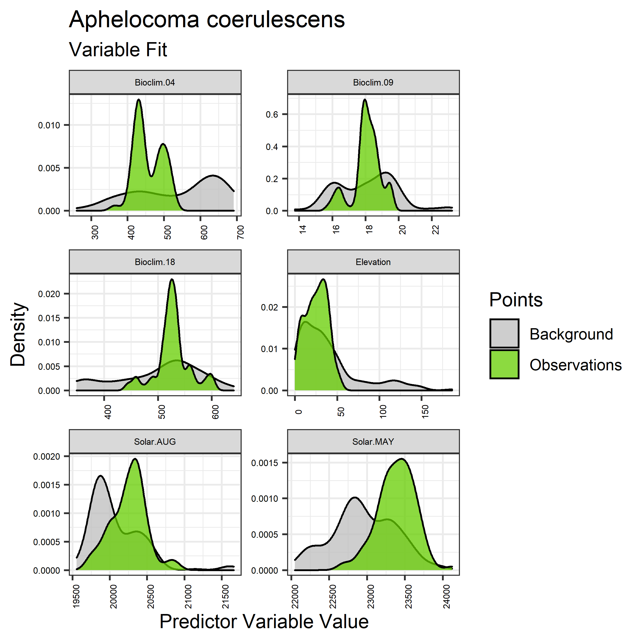
Figure 5. Sampling of continuous predictor variables retained in the best-fit Aphelocoma coerulescens distribution models. Distribution of each variable at points of species occurrence (green) are contrasted with points sampled across the full modeled extent (gray).
|
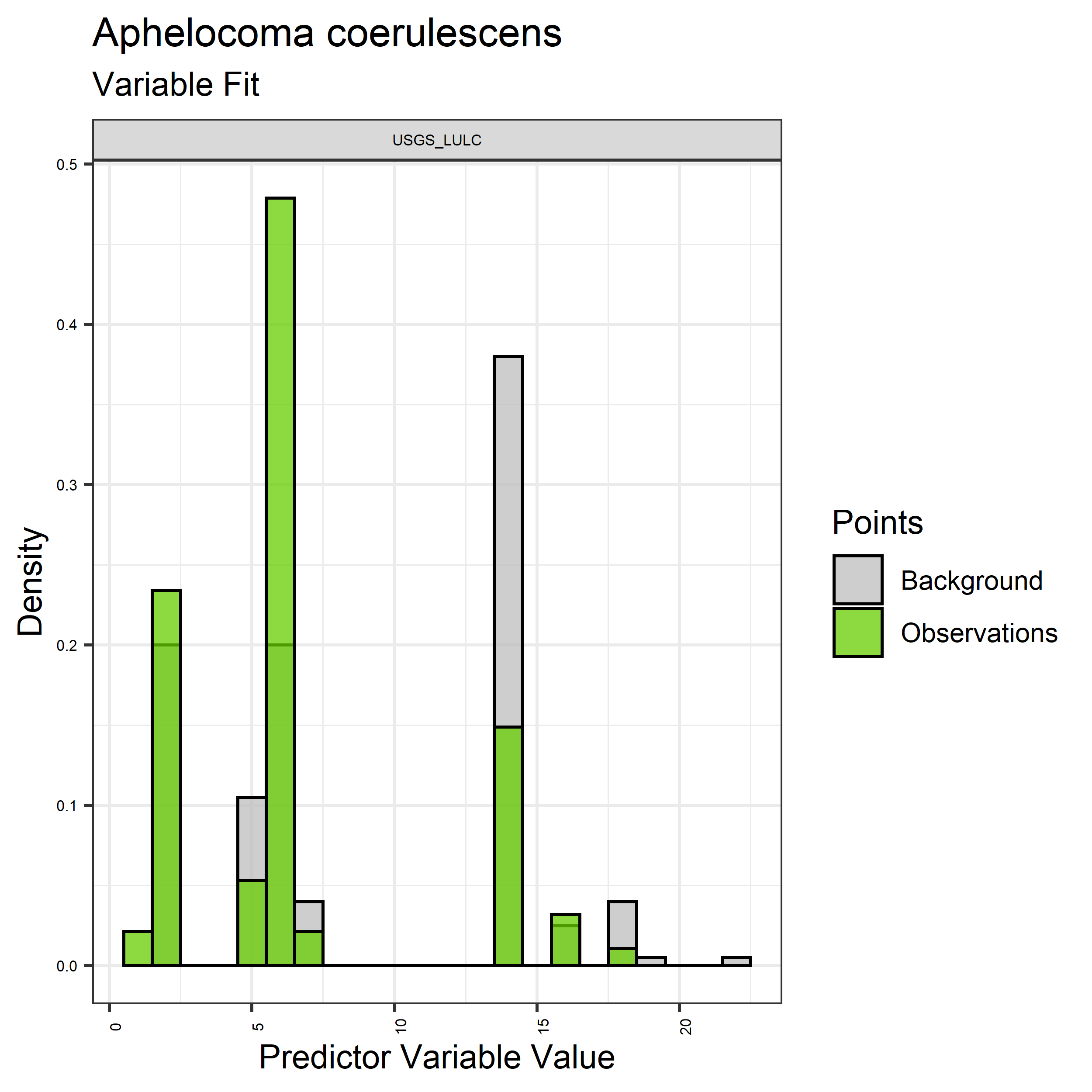
Figure 6. Sampling of discrete predictor variables retained in the best-fit Aphelocoma coerulescens distribution models. Distribution of each variable at points of species occurrence (green) are contrasted with points sampled across the full modeled extent.
|
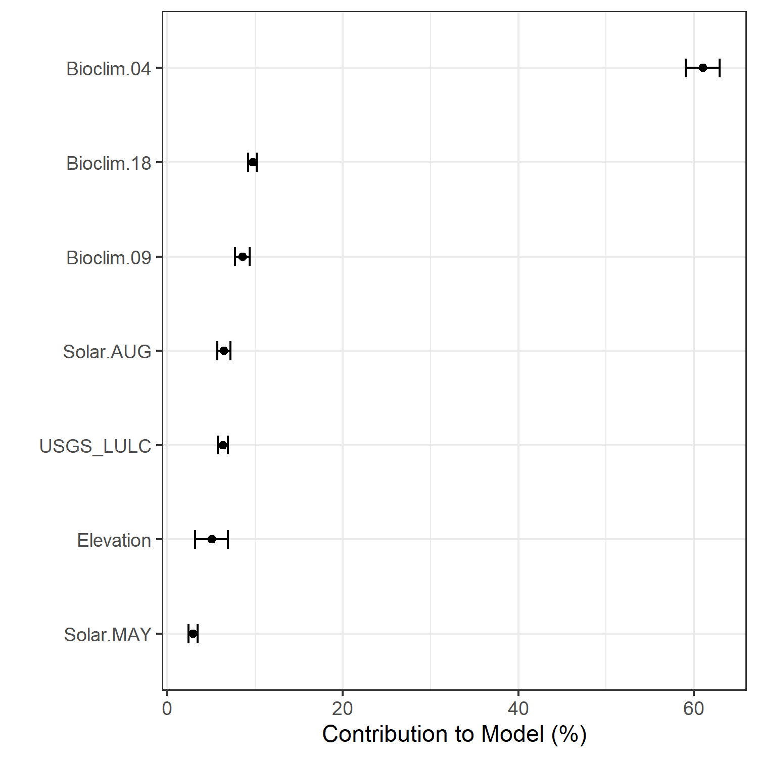
Figure 7. Percent contribution of each variable to best-fit species distribution models for Aphelocoma coerulescens. Values sum to 1.0.
|
Table 6. Mean Area Under Curve (AUC) for five realizations of the best-fit SDM for Aphelocoma coerulescens, calculated using 20% of species location records reserved for final evaluation.
| V1 |
V2 |
V3 |
V4 |
V5 |
mean |
sd |
| 0.912021 |
0.911543 |
0.912766 |
0.91516 |
0.914096 |
0.913117 |
0.001076 |
|
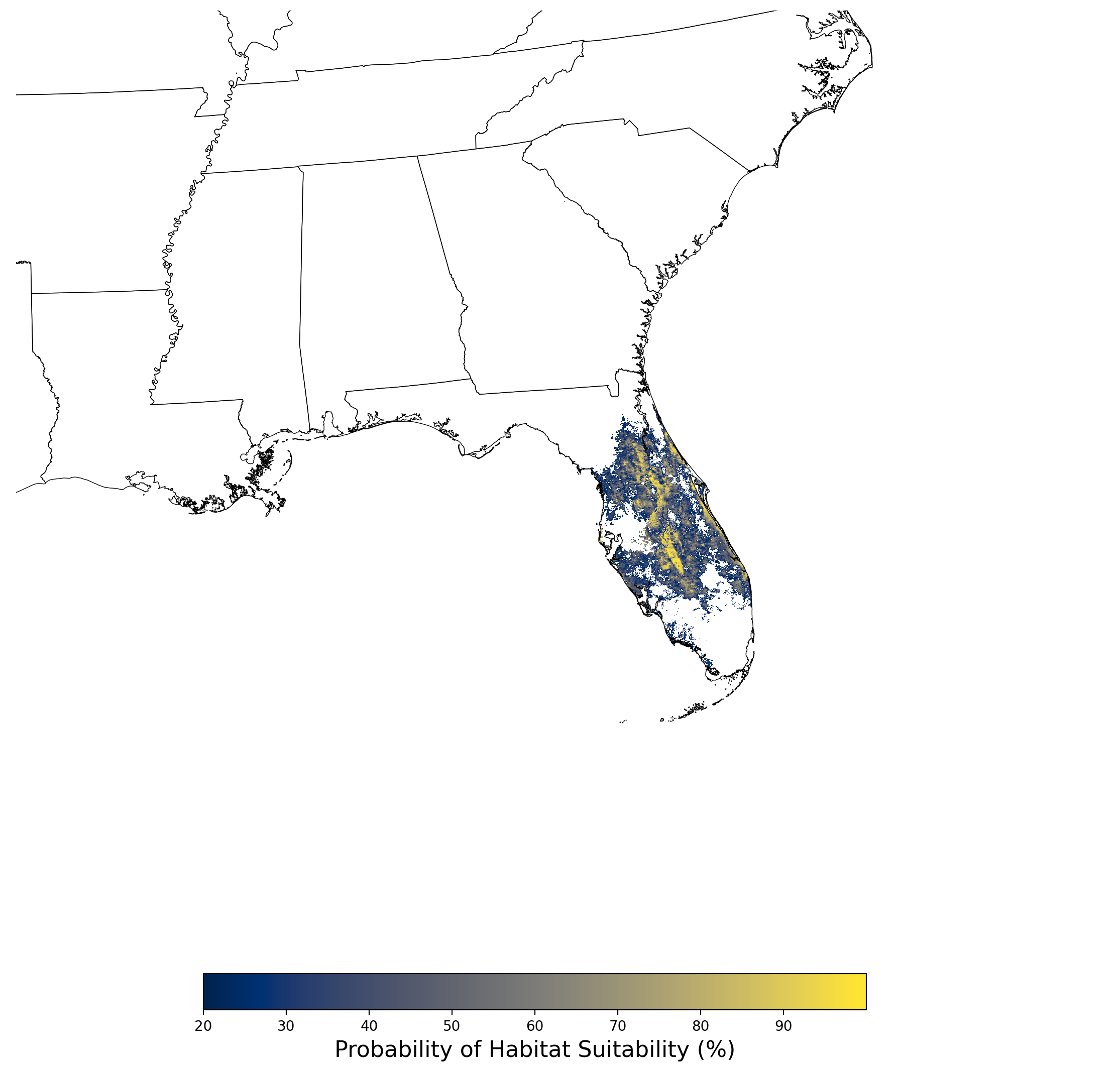
Figure 8. Final mean SDM output for Aphelocoma coerulescens. |
2.2.2 Species Distribution Modeling Results - Bombus affinis
The species distribution modeling results consist of the following figures and tables:
- A table showing the SDM inputs (Table 7)
- A map showing the extent of SDM coverage (Figure 9)
- A graph showing the correlation between the predictor variable selected for evaluation (Figure 10)
- A graph of the model fit of each SDM iteration as measured by total Area Under Curve (AUC) where the curve is the Receiver Operating Curve, based on training data (Figure 11)
- A table showing the diagnostic statistics of the training data used in the final selected SDM iteration (Table 8)
- Graphs illustrating the predictor variable values sampled by the species observations and randomly selected background locations for continuous variables (Figure 12), and discrete variables (Figure 13)
- A graph showing the percent contribution of each predictor variable to the final selected SDM (Figure 14)
- A table showing the mean AUC for each of the five model runs that are averaged for the final selected SDM (Table 9)
- A map of the final averaged SDM (Figure 15)
Table 7. Input parameters for species distribution modeling of Bombus affinis.
| Number of predictors |
33 |
| Names of predictors |
Bioclim.01.tif, Bioclim.02.tif, Bioclim.03.tif, Bioclim.04.tif,
Bioclim.05.tif, Bioclim.06.tif, Bioclim.07.tif, Bioclim.08.tif,
Bioclim.09.tif, Bioclim.10.tif, Bioclim.11.tif, Bioclim.12.tif,
Bioclim.13.tif, Bioclim.14.tif, Bioclim.15.tif, Bioclim.16.tif,
Bioclim.17.tif, Bioclim.18.tif, Bioclim.19.tif, Elevation.tif,
Solar.APR.tif, Solar.AUG.tif, Solar.DEC.tif, Solar.FEB.tif,
Solar.JAN.tif, Solar.JUL.tif, Solar.JUN.tif, Solar.MAR.tif,
Solar.MAY.tif, Solar.NOV.tif, Solar.OCT.tif, Solar.SEP.tif,
USGS_LULC.tif |
| Predictor correlation threshold |
0.67 |
| Predictor contribution threshold |
1.0 |
| SDM threshold |
0.2 |
| Number of iterations conducted |
3 |
| Final SDM iteration number |
2 |
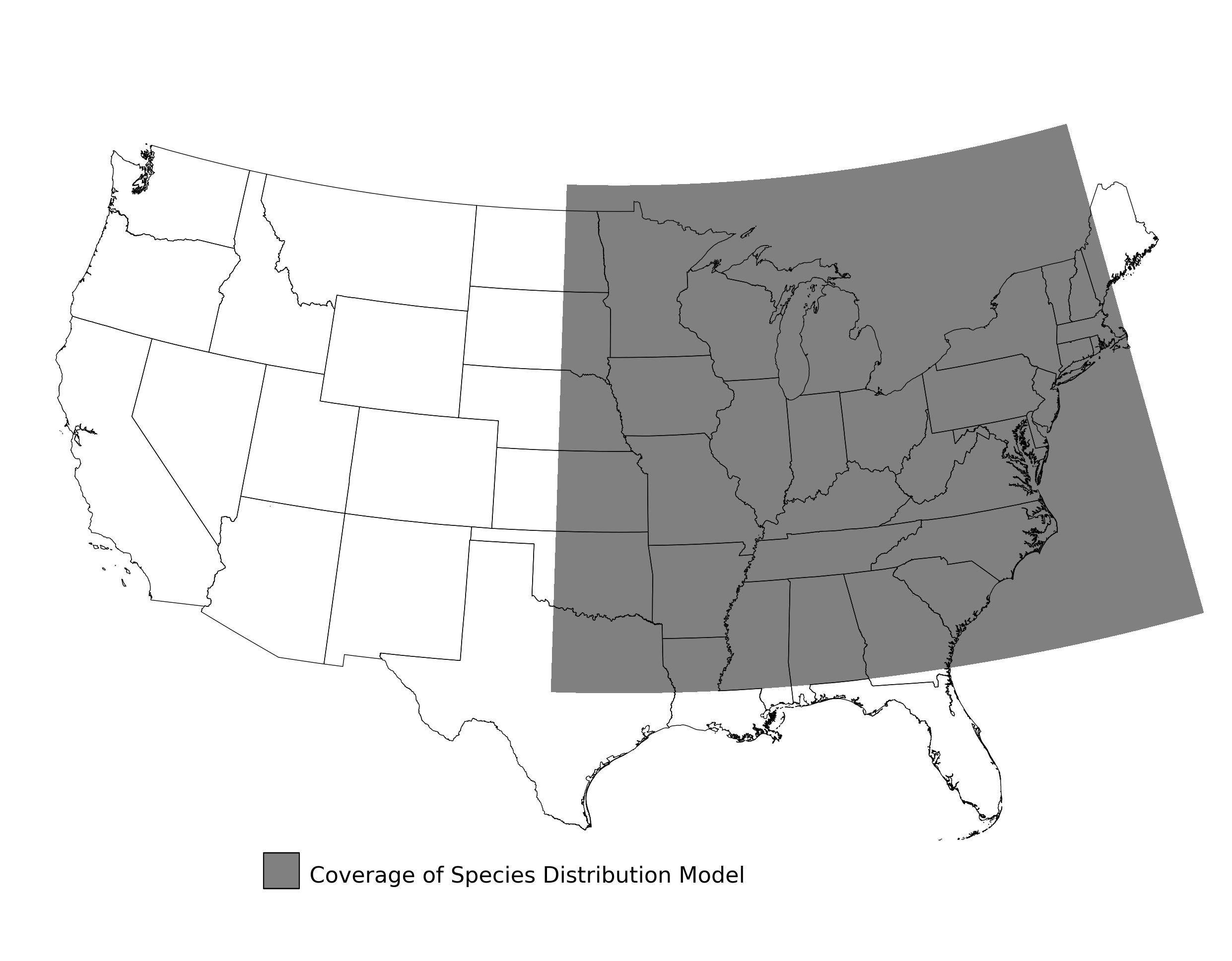
Figure 9. Extent of the species range modeled for Bombus affinis. Modeling extent is determined by buffering species location records in all directions by 3 degrees latitude/longitude.
|
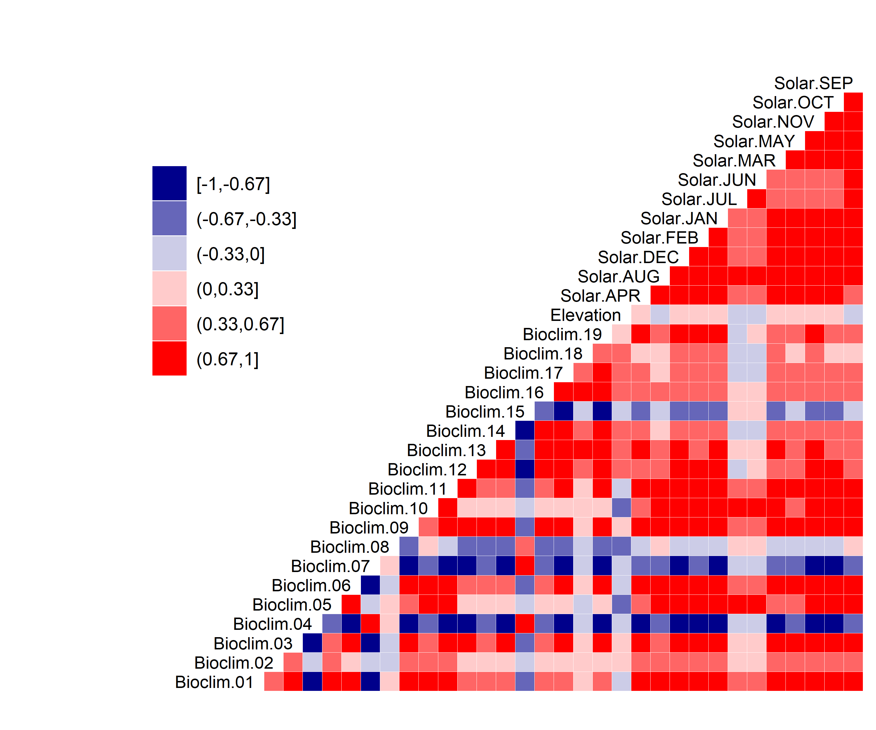
Figure 10. Correlation between SDM predictor variables for Bombus affinis.
|
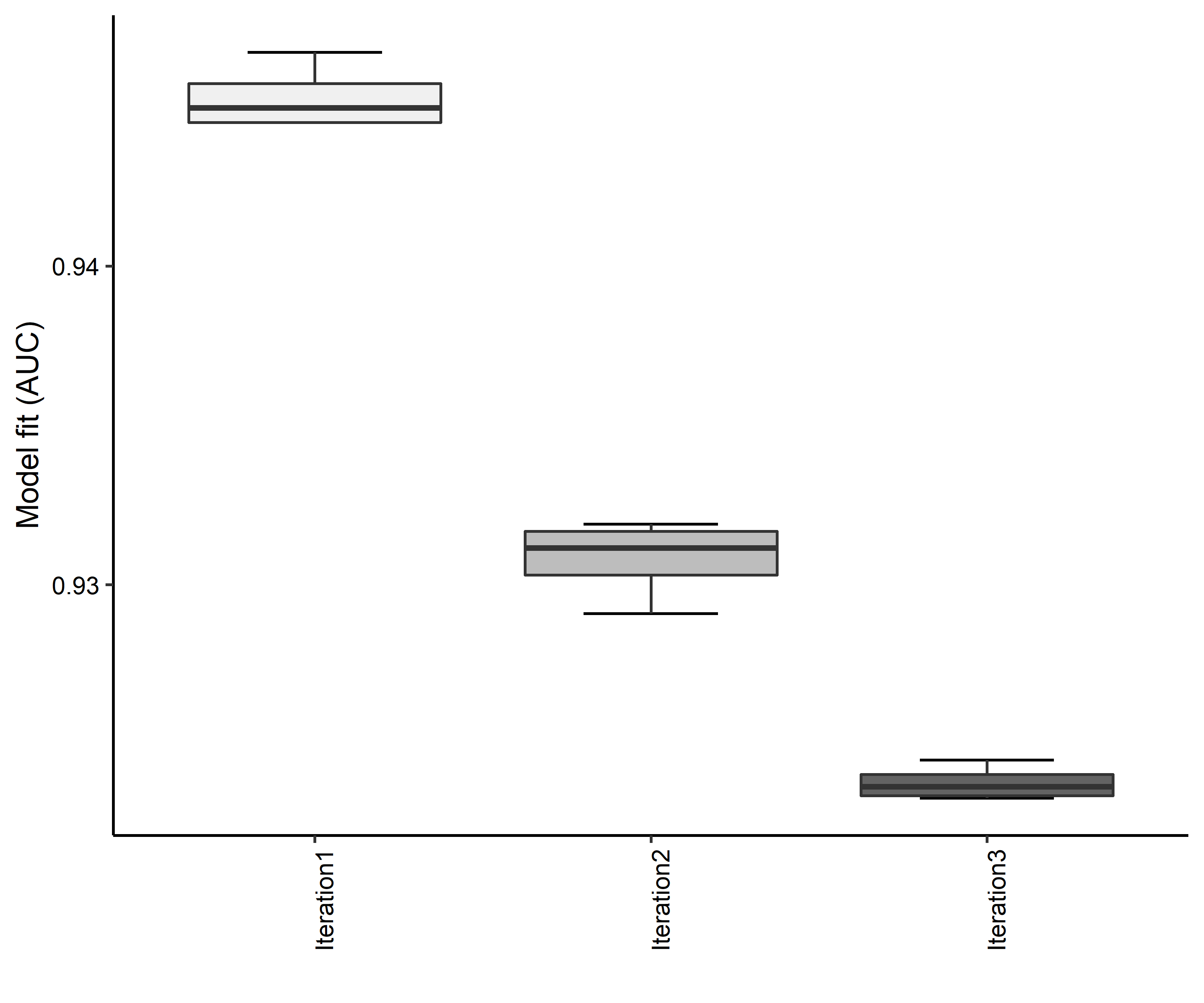
Figure 11. Boxplots of model fit for each iteration of Bombus affinis distribution modeling. Statistics are calculated using 80% of species location records reserved for model training.
|
Table 8. Diagnostic statistics of the training data used in SDM iteration #2 for Bombus affinis.
| Model Output |
Realization 1 |
Realization 2 |
Realization 3 |
Realization 4 |
Realization 5 |
Mean |
Standard Deviation |
| Number of training samples |
482.0000 |
482.0000 |
482.0000 |
482.0000 |
482.0000 |
482.00000 |
0.000000 |
| Regularized training gain |
1.5694 |
1.5323 |
1.5550 |
1.5731 |
1.5673 |
1.55942 |
0.016612 |
| Unregularized training gain |
1.7028 |
1.6640 |
1.6844 |
1.7079 |
1.6979 |
1.69140 |
0.017637 |
| Iterations |
500.0000 |
500.0000 |
500.0000 |
500.0000 |
500.0000 |
500.00000 |
0.000000 |
| Training AUC |
0.9316 |
0.9291 |
0.9307 |
0.9319 |
0.9316 |
0.93098 |
0.001143 |
| Number of background points |
10482.0000 |
10482.0000 |
10482.0000 |
10482.0000 |
10482.0000 |
10482.00000 |
0.000000 |
| Bioclim 02 contribution |
3.4019 |
3.4588 |
4.2127 |
3.1648 |
3.7208 |
3.59180 |
0.399449 |
| Bioclim 17 contribution |
9.6448 |
10.1532 |
10.9534 |
9.5237 |
11.0522 |
10.26546 |
0.714187 |
| Elevation contribution |
9.8351 |
7.7513 |
11.7720 |
14.5770 |
10.4620 |
10.87948 |
2.525806 |
| Solar SEP contribution |
44.0121 |
44.6700 |
41.0784 |
36.8036 |
44.4008 |
42.19298 |
3.339424 |
| USGS_LULC contribution |
33.1060 |
33.9666 |
31.9835 |
35.9310 |
30.3642 |
33.07026 |
2.091192 |
| Bioclim 02 permutation importance |
7.7642 |
6.6776 |
6.7047 |
7.1052 |
8.4193 |
7.33420 |
0.748695 |
| Bioclim 17 permutation importance |
9.4948 |
9.7107 |
8.3938 |
9.1045 |
10.8761 |
9.51598 |
0.910617 |
| Elevation permutation importance |
4.6518 |
4.0538 |
5.6120 |
6.4124 |
5.6717 |
5.28034 |
0.927926 |
| Solar SEP permutation importance |
68.0149 |
69.2487 |
68.0498 |
66.6316 |
66.0383 |
67.59666 |
1.271743 |
| USGS_LULC permutation importance |
10.0744 |
10.3091 |
11.2397 |
10.7462 |
8.9947 |
10.27282 |
0.841609 |
| Entropy |
7.6861 |
7.7266 |
7.7078 |
7.6899 |
7.6927 |
7.70062 |
0.016696 |
| Prevalence average probability of presence over background sites |
0.1177 |
0.1228 |
0.1205 |
0.1182 |
0.1186 |
0.11956 |
0.002098 |
| Fixed cumulative value 1 cumulative threshold |
1.0000 |
1.0000 |
1.0000 |
1.0000 |
1.0000 |
1.00000 |
0.000000 |
| Fixed cumulative value 1 Cloglog threshold |
0.0166 |
0.0175 |
0.0182 |
0.0165 |
0.0176 |
0.01728 |
0.000719 |
| Fixed cumulative value 1 area |
0.5230 |
0.5337 |
0.5210 |
0.5300 |
0.5204 |
0.52562 |
0.005915 |
| Fixed cumulative value 1 training omission |
0.0021 |
0.0021 |
0.0021 |
0.0021 |
0.0021 |
0.00210 |
0.000000 |
| Fixed cumulative value 5 cumulative threshold |
5.0000 |
5.0000 |
5.0000 |
5.0000 |
5.0000 |
5.00000 |
0.000000 |
| Fixed cumulative value 5 Cloglog threshold |
0.0712 |
0.0731 |
0.0737 |
0.0724 |
0.0738 |
0.07284 |
0.001074 |
| Fixed cumulative value 5 area |
0.3096 |
0.3226 |
0.3148 |
0.3148 |
0.3131 |
0.31498 |
0.004759 |
| Fixed cumulative value 5 training omission |
0.0353 |
0.0353 |
0.0373 |
0.0353 |
0.0332 |
0.03528 |
0.001450 |
| Fixed cumulative value 10 cumulative threshold |
10.0000 |
10.0000 |
10.0000 |
10.0000 |
10.0000 |
10.00000 |
0.000000 |
| Fixed cumulative value 10 Cloglog threshold |
0.1413 |
0.1435 |
0.1462 |
0.1394 |
0.1411 |
0.14230 |
0.002622 |
| Fixed cumulative value 10 area |
0.2127 |
0.2238 |
0.2188 |
0.2165 |
0.2172 |
0.21780 |
0.004033 |
| Fixed cumulative value 10 training omission |
0.0664 |
0.0685 |
0.0685 |
0.0643 |
0.0685 |
0.06724 |
0.001878 |
| Minimum training presence cumulative threshold |
0.4555 |
0.4662 |
0.5989 |
0.4525 |
0.5387 |
0.50236 |
0.064479 |
| Minimum training presence Cloglog threshold |
0.0084 |
0.0091 |
0.0111 |
0.0082 |
0.0101 |
0.00938 |
0.001215 |
| Minimum training presence area |
0.6172 |
0.6228 |
0.5798 |
0.6257 |
0.5908 |
0.60726 |
0.020648 |
| Minimum training presence training omission |
0.0000 |
0.0000 |
0.0000 |
0.0000 |
0.0000 |
0.00000 |
0.000000 |
| X10 percentile training presence cumulative threshold |
14.3467 |
15.6674 |
14.9150 |
15.4622 |
14.3757 |
14.95340 |
0.606624 |
| X10 percentile training presence Cloglog threshold |
0.2173 |
0.2348 |
0.2304 |
0.2318 |
0.2181 |
0.22648 |
0.008176 |
| X10 percentile training presence area |
0.1660 |
0.1645 |
0.1680 |
0.1596 |
0.1699 |
0.16560 |
0.003925 |
| X10 percentile training presence training omission |
0.0996 |
0.0996 |
0.0996 |
0.0996 |
0.0996 |
0.09960 |
0.000000 |
| Equal training sensitivity and specificity cumulative threshold |
19.7729 |
20.7749 |
20.7442 |
20.1557 |
20.0090 |
20.29134 |
0.448834 |
| Equal training sensitivity and specificity Cloglog threshold |
0.3088 |
0.3154 |
0.3163 |
0.3147 |
0.3046 |
0.31196 |
0.005058 |
| Equal training sensitivity and specificity area |
0.1286 |
0.1300 |
0.1286 |
0.1286 |
0.1307 |
0.12930 |
0.000990 |
| Equal training sensitivity and specificity training omission |
0.1286 |
0.1307 |
0.1286 |
0.1286 |
0.1307 |
0.12944 |
0.001150 |
| Maximum training sensitivity plus specificity cumulative threshold |
20.3764 |
20.7582 |
21.5525 |
20.1557 |
22.1775 |
21.00406 |
0.844374 |
| Maximum training sensitivity plus specificity Cloglog threshold |
0.3181 |
0.3154 |
0.3296 |
0.3147 |
0.3420 |
0.32396 |
0.011733 |
| Maximum training sensitivity plus specificity area |
0.1252 |
0.1300 |
0.1242 |
0.1286 |
0.1192 |
0.12544 |
0.004222 |
| Maximum training sensitivity plus specificity training omission |
0.1286 |
0.1286 |
0.1307 |
0.1266 |
0.1390 |
0.13070 |
0.004861 |
| Balance training omission predicted area and threshold value cumulative threshold |
2.1122 |
2.8113 |
2.2573 |
2.3783 |
2.6306 |
2.43794 |
0.282316 |
| Balance training omission predicted area and threshold value Cloglog threshold |
0.0328 |
0.0443 |
0.0363 |
0.0360 |
0.0409 |
0.03806 |
0.004528 |
| Balance training omission predicted area and threshold value area |
0.4274 |
0.4024 |
0.4220 |
0.4169 |
0.3996 |
0.41366 |
0.012179 |
| Balance training omission predicted area and threshold value training omission |
0.0104 |
0.0166 |
0.0104 |
0.0124 |
0.0124 |
0.01244 |
0.002531 |
| Equate entropy of thresholded and original distributions cumulative threshold |
10.3831 |
10.5621 |
10.5054 |
10.5972 |
10.6189 |
10.53334 |
0.094311 |
| Equate entropy of thresholded and original distributions Cloglog threshold |
0.1471 |
0.1534 |
0.1559 |
0.1482 |
0.1517 |
0.15126 |
0.003639 |
| Equate entropy of thresholded and original distributions area |
0.2077 |
0.2163 |
0.2123 |
0.2085 |
0.2091 |
0.21078 |
0.003546 |
| Equate entropy of thresholded and original distributions training omission |
0.0705 |
0.0726 |
0.0705 |
0.0705 |
0.0726 |
0.07134 |
0.001150 |
|
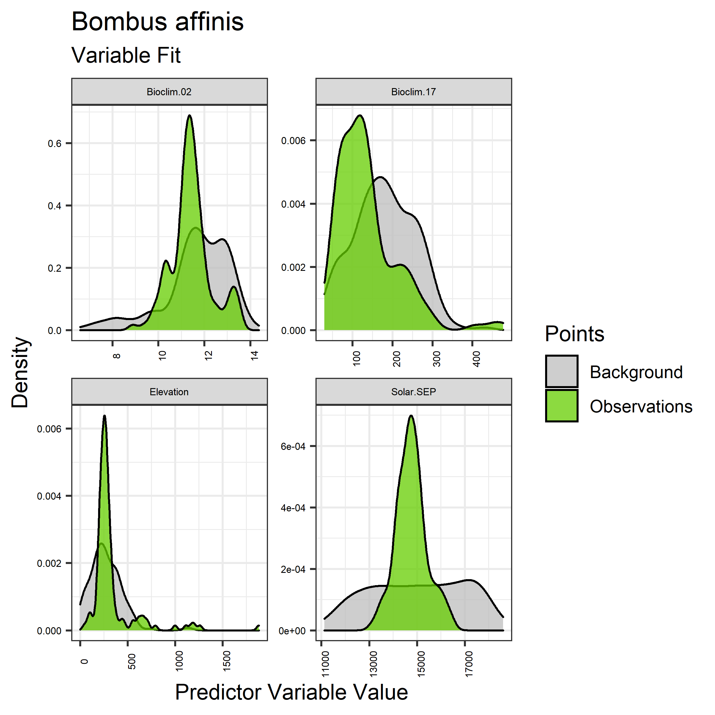
Figure 12. Sampling of continuous predictor variables retained in the best-fit Bombus affinis distribution models. Distribution of each variable at points of species occurrence (green) are contrasted with points sampled across the full modeled extent (gray).
|
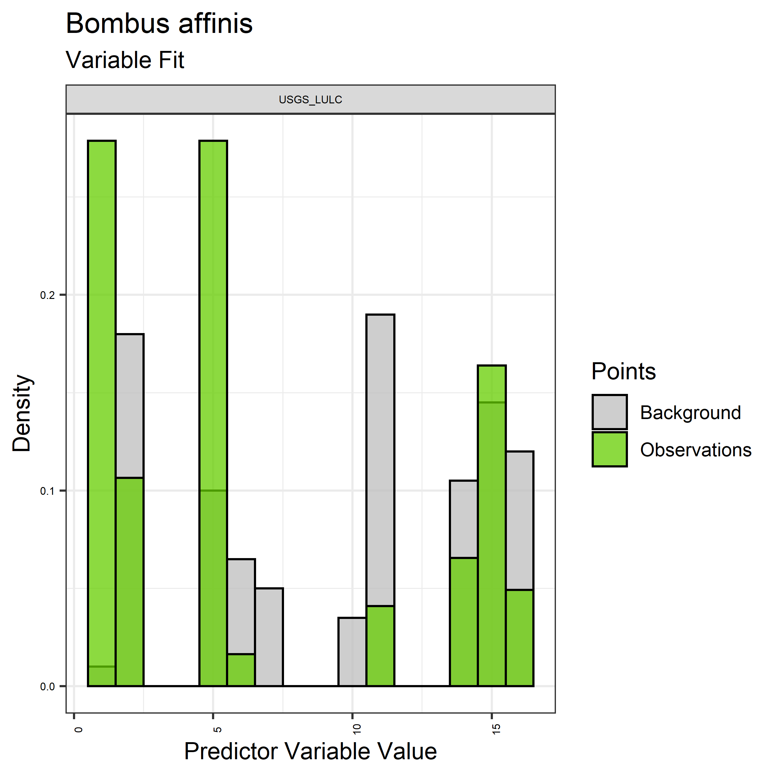
Figure 13. Sampling of discrete predictor variables retained in the best-fit Bombus affinis distribution models. Distribution of each variable at points of species occurrence (green) are contrasted with points sampled across the full modeled extent.
|
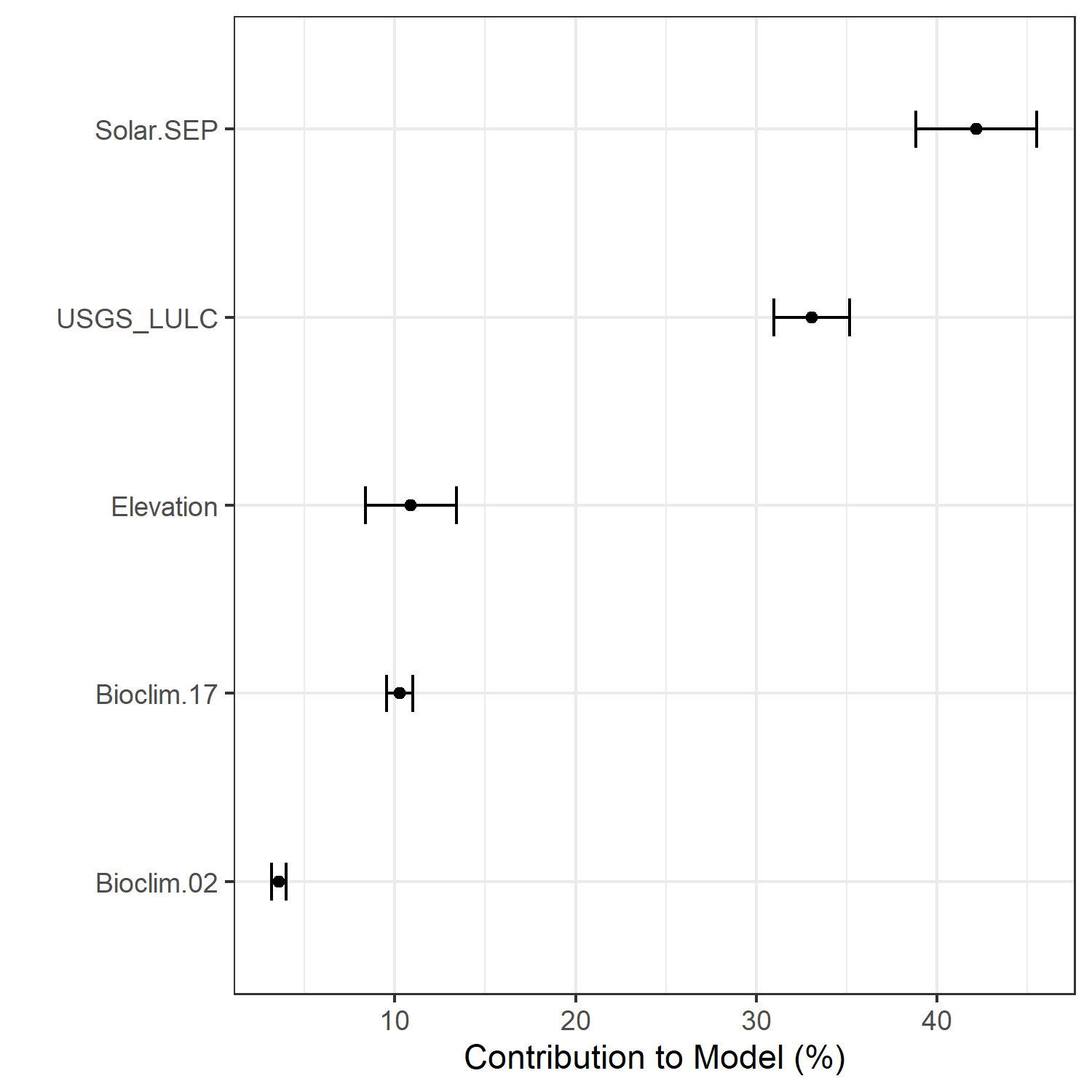
Figure 14. Percent contribution of each variable to best-fit species distribution models for Bombus affinis. Values sum to 1.0.
|
Table 9. Mean Area Under Curve (AUC) for five realizations of the best-fit SDM for Bombus affinis, calculated using 20% of species location records reserved for final evaluation.
| V1 |
V2 |
V3 |
V4 |
V5 |
mean |
sd |
| 0.93959 |
0.939713 |
0.941598 |
0.940984 |
0.94123 |
0.940623 |
0.000411 |
|
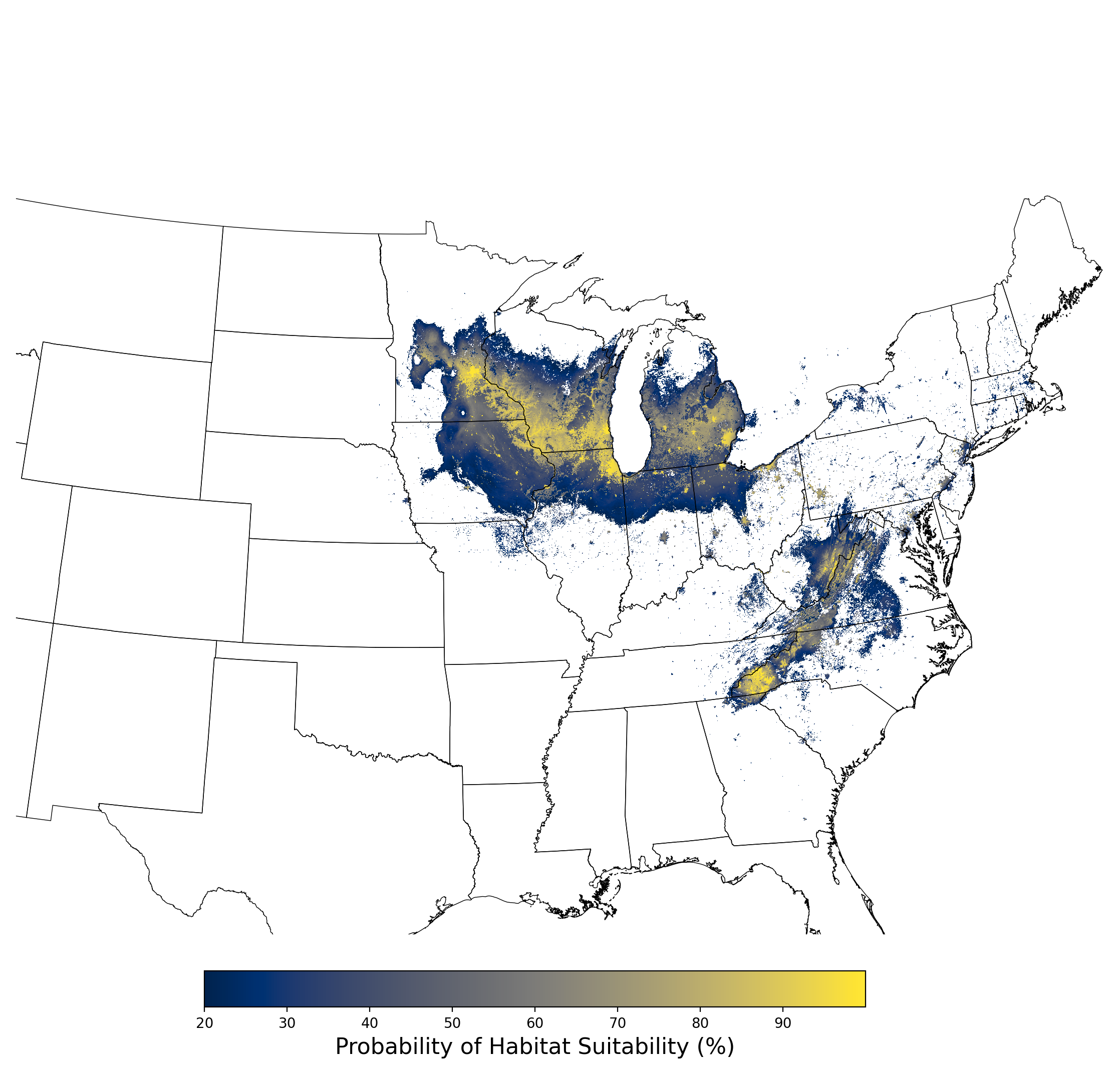
Figure 15. Final mean SDM output for Bombus affinis. |
2.2.3 Species Distribution Modeling Results for Bufo houstonensis
The species distribution modeling results consist of the following figures and tables:
- A table showing the SDM inputs (Table 10)
- A map showing the extent of SDM coverage (Figure 16)
- A graph showing the correlation between the predictor variable selected for evaluation (Figure 17)
- A graph of the model fit of each SDM iteration as measured by total Area Under Curve (AUC) where the curve is the Receiver Operating Curve, based on training data (Figure 18)
- A table showing the diagnostic statistics of the training data used in the final selected SDM iteration (Table 11)
- Graphs illustrating the predictor variable values sampled by the species observations and randomly selected background locations for continuous variables (Figure 19), and discrete variables (Figure 20)
- A graph showing the percent contribution of each predictor variable to the final selected SDM (Figure 21)
- A table showing the mean AUC for each of the five model runs that are averaged for the final selected SDM (Table 12)
- A map of the final averaged SDM (Figure 22)
Table 10. Input parameters for species distribution modeling of Bufo houstonensis.
| Number of predictors |
33 |
| Names of predictors |
Bioclim.01.tif, Bioclim.02.tif, Bioclim.03.tif, Bioclim.04.tif,
Bioclim.05.tif, Bioclim.06.tif, Bioclim.07.tif, Bioclim.08.tif,
Bioclim.09.tif, Bioclim.10.tif, Bioclim.11.tif, Bioclim.12.tif,
Bioclim.13.tif, Bioclim.14.tif, Bioclim.15.tif, Bioclim.16.tif,
Bioclim.17.tif, Bioclim.18.tif, Bioclim.19.tif, Elevation.tif,
Solar.APR.tif, Solar.AUG.tif, Solar.DEC.tif, Solar.FEB.tif,
Solar.JAN.tif, Solar.JUL.tif, Solar.JUN.tif, Solar.MAR.tif,
Solar.MAY.tif, Solar.NOV.tif, Solar.OCT.tif, Solar.SEP.tif,
USGS_LULC.tif |
| Predictor correlation threshold |
0.67 |
| Predictor contribution threshold |
1.0 |
| SDM threshold |
0.2 |
| Number of iterations conducted |
4 |
| Final SDM iteration number |
3 |
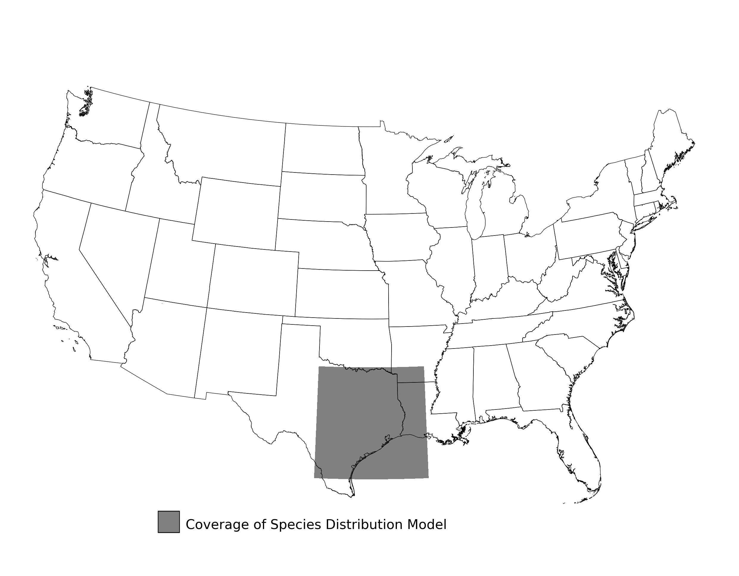
Figure 16. Extent of the species range modeled for Bufo houstonensis. Modeling extent is determined by buffering species location records in all directions by 3 degrees latitude/longitude.
|
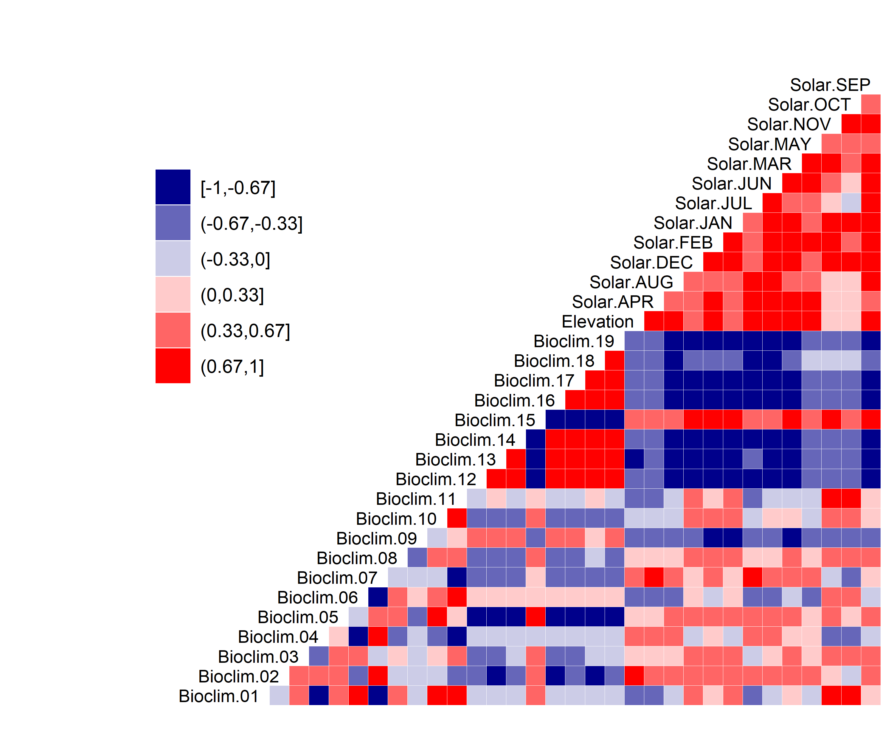
Figure 17. Correlation between SDM predictor variables for Bufo houstonensis.
|
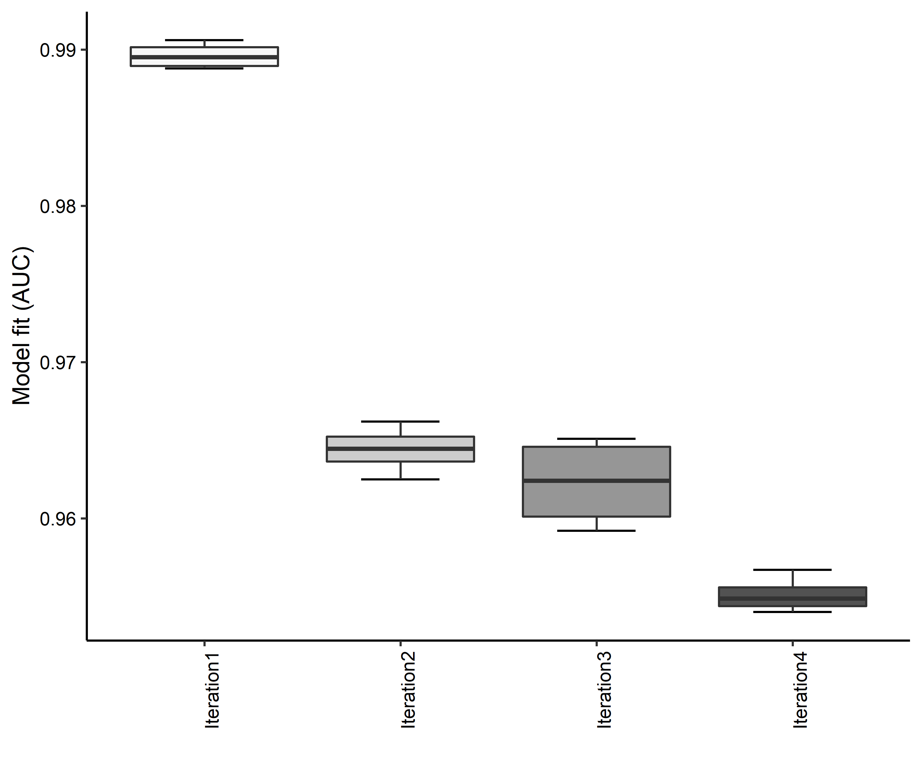
Figure 18. Boxplots of model fit for each iteration of Bufo houstonensis distribution modeling. Statistics are calculated using 80% of species location records reserved for model training.
|
Table 11. Diagnostic statistics of the training data used in SDM iteration #3 for Bufo houstonensis.
| Model Output |
Realization 1 |
Realization 2 |
Realization 3 |
Realization 4 |
Realization 5 |
Mean |
Standard Deviation |
| Number of training samples |
22.0000 |
22.0000 |
22.0000 |
22.0000 |
22.0000 |
22.00000 |
0.000000 |
| Regularized training gain |
1.5429 |
1.6155 |
1.5428 |
1.6138 |
1.5289 |
1.56878 |
0.042263 |
| Unregularized training gain |
2.1446 |
2.2561 |
2.1545 |
2.2348 |
2.1389 |
2.18578 |
0.055272 |
| Iterations |
400.0000 |
500.0000 |
420.0000 |
420.0000 |
420.0000 |
432.00000 |
38.987177 |
| Training AUC |
0.9612 |
0.9651 |
0.9592 |
0.9644 |
0.9604 |
0.96206 |
0.002569 |
| Number of background points |
10021.0000 |
10016.0000 |
10020.0000 |
10021.0000 |
10022.0000 |
10020.00000 |
2.345208 |
| Bioclim 11 contribution |
30.2334 |
32.0528 |
29.2680 |
30.4041 |
30.5948 |
30.51062 |
1.002211 |
| Bioclim 17 contribution |
47.4778 |
49.0326 |
49.0516 |
48.3420 |
47.4080 |
48.26240 |
0.801245 |
| USGS_LULC contribution |
22.2888 |
18.9146 |
21.6805 |
21.2538 |
21.9973 |
21.22700 |
1.348551 |
| Bioclim 11 permutation importance |
45.9006 |
31.8002 |
31.1550 |
32.9369 |
38.8273 |
36.12400 |
6.253670 |
| Bioclim 17 permutation importance |
48.2827 |
65.2166 |
58.7453 |
59.2480 |
52.0999 |
56.71850 |
6.618500 |
| USGS_LULC permutation importance |
5.8167 |
2.9832 |
10.0997 |
7.8151 |
9.0728 |
7.15750 |
2.827538 |
| Entropy |
7.6672 |
7.5941 |
7.6703 |
7.5981 |
7.6831 |
7.64256 |
0.042852 |
| Prevalence average probability of presence over background sites |
0.1235 |
0.1153 |
0.1241 |
0.1151 |
0.1256 |
0.12072 |
0.005097 |
| Fixed cumulative value 1 cumulative threshold |
1.0000 |
1.0000 |
1.0000 |
1.0000 |
1.0000 |
1.00000 |
0.000000 |
| Fixed cumulative value 1 Cloglog threshold |
0.0194 |
0.0187 |
0.0199 |
0.0188 |
0.0203 |
0.01942 |
0.000691 |
| Fixed cumulative value 1 area |
0.4446 |
0.4093 |
0.4396 |
0.4203 |
0.4392 |
0.43060 |
0.015089 |
| Fixed cumulative value 1 training omission |
0.0000 |
0.0000 |
0.0000 |
0.0000 |
0.0000 |
0.00000 |
0.000000 |
| Fixed cumulative value 5 cumulative threshold |
5.0000 |
5.0000 |
5.0000 |
5.0000 |
5.0000 |
5.00000 |
0.000000 |
| Fixed cumulative value 5 Cloglog threshold |
0.0975 |
0.1027 |
0.0958 |
0.0945 |
0.1000 |
0.09810 |
0.003293 |
| Fixed cumulative value 5 area |
0.2662 |
0.2415 |
0.2609 |
0.2506 |
0.2660 |
0.25704 |
0.010748 |
| Fixed cumulative value 5 training omission |
0.0000 |
0.0000 |
0.0000 |
0.0000 |
0.0000 |
0.00000 |
0.000000 |
| Fixed cumulative value 10 cumulative threshold |
10.0000 |
10.0000 |
10.0000 |
10.0000 |
10.0000 |
10.00000 |
0.000000 |
| Fixed cumulative value 10 Cloglog threshold |
0.1955 |
0.2054 |
0.2014 |
0.1978 |
0.2094 |
0.20190 |
0.005624 |
| Fixed cumulative value 10 area |
0.1964 |
0.1796 |
0.1918 |
0.1850 |
0.1979 |
0.19014 |
0.007741 |
| Fixed cumulative value 10 training omission |
0.0000 |
0.0000 |
0.0000 |
0.0000 |
0.0000 |
0.00000 |
0.000000 |
| Minimum training presence cumulative threshold |
14.3492 |
13.5305 |
12.9116 |
14.1465 |
13.5961 |
13.70678 |
0.566059 |
| Minimum training presence Cloglog threshold |
0.2750 |
0.2776 |
0.2624 |
0.2698 |
0.2727 |
0.27150 |
0.005844 |
| Minimum training presence area |
0.1613 |
0.1540 |
0.1680 |
0.1538 |
0.1695 |
0.16132 |
0.007444 |
| Minimum training presence training omission |
0.0000 |
0.0000 |
0.0000 |
0.0000 |
0.0000 |
0.00000 |
0.000000 |
| X10 percentile training presence cumulative threshold |
22.0619 |
28.9459 |
21.1269 |
20.8289 |
20.9710 |
22.78692 |
3.476556 |
| X10 percentile training presence Cloglog threshold |
0.3941 |
0.4930 |
0.3992 |
0.3704 |
0.3743 |
0.40620 |
0.050072 |
| X10 percentile training presence area |
0.1206 |
0.0909 |
0.1247 |
0.1196 |
0.1287 |
0.11690 |
0.014975 |
| X10 percentile training presence training omission |
0.0909 |
0.0909 |
0.0909 |
0.0909 |
0.0909 |
0.09090 |
0.000000 |
| Equal training sensitivity and specificity cumulative threshold |
22.0619 |
28.9117 |
21.1507 |
20.8289 |
20.9926 |
22.78916 |
3.455763 |
| Equal training sensitivity and specificity Cloglog threshold |
0.3941 |
0.4930 |
0.3994 |
0.3704 |
0.3743 |
0.40624 |
0.050065 |
| Equal training sensitivity and specificity area |
0.1206 |
0.0910 |
0.1247 |
0.1196 |
0.1287 |
0.11692 |
0.014932 |
| Equal training sensitivity and specificity training omission |
0.1364 |
0.0909 |
0.1364 |
0.1364 |
0.1364 |
0.12730 |
0.020348 |
| Maximum training sensitivity plus specificity cumulative threshold |
14.3492 |
13.5305 |
12.9116 |
14.1465 |
13.5961 |
13.70678 |
0.566059 |
| Maximum training sensitivity plus specificity Cloglog threshold |
0.2750 |
0.2776 |
0.2624 |
0.2698 |
0.2727 |
0.27150 |
0.005844 |
| Maximum training sensitivity plus specificity area |
0.1613 |
0.1540 |
0.1680 |
0.1538 |
0.1695 |
0.16132 |
0.007444 |
| Maximum training sensitivity plus specificity training omission |
0.0000 |
0.0000 |
0.0000 |
0.0000 |
0.0000 |
0.00000 |
0.000000 |
| Balance training omission predicted area and threshold value cumulative threshold |
4.2936 |
3.9502 |
4.2376 |
3.9819 |
4.1939 |
4.13144 |
0.155465 |
| Balance training omission predicted area and threshold value Cloglog threshold |
0.0817 |
0.0762 |
0.0820 |
0.0764 |
0.0828 |
0.07982 |
0.003239 |
| Balance training omission predicted area and threshold value area |
0.2823 |
0.2638 |
0.2784 |
0.2735 |
0.2844 |
0.27648 |
0.008215 |
| Balance training omission predicted area and threshold value training omission |
0.0000 |
0.0000 |
0.0000 |
0.0000 |
0.0000 |
0.00000 |
0.000000 |
| Equate entropy of thresholded and original distributions cumulative threshold |
8.4409 |
8.0717 |
7.9470 |
8.6002 |
8.2036 |
8.25268 |
0.266833 |
| Equate entropy of thresholded and original distributions Cloglog threshold |
0.1672 |
0.1675 |
0.1602 |
0.1682 |
0.1684 |
0.16630 |
0.003445 |
| Equate entropy of thresholded and original distributions area |
0.2132 |
0.1983 |
0.2139 |
0.1990 |
0.2166 |
0.20820 |
0.008813 |
| Equate entropy of thresholded and original distributions training omission |
0.0000 |
0.0000 |
0.0000 |
0.0000 |
0.0000 |
0.00000 |
0.000000 |
|
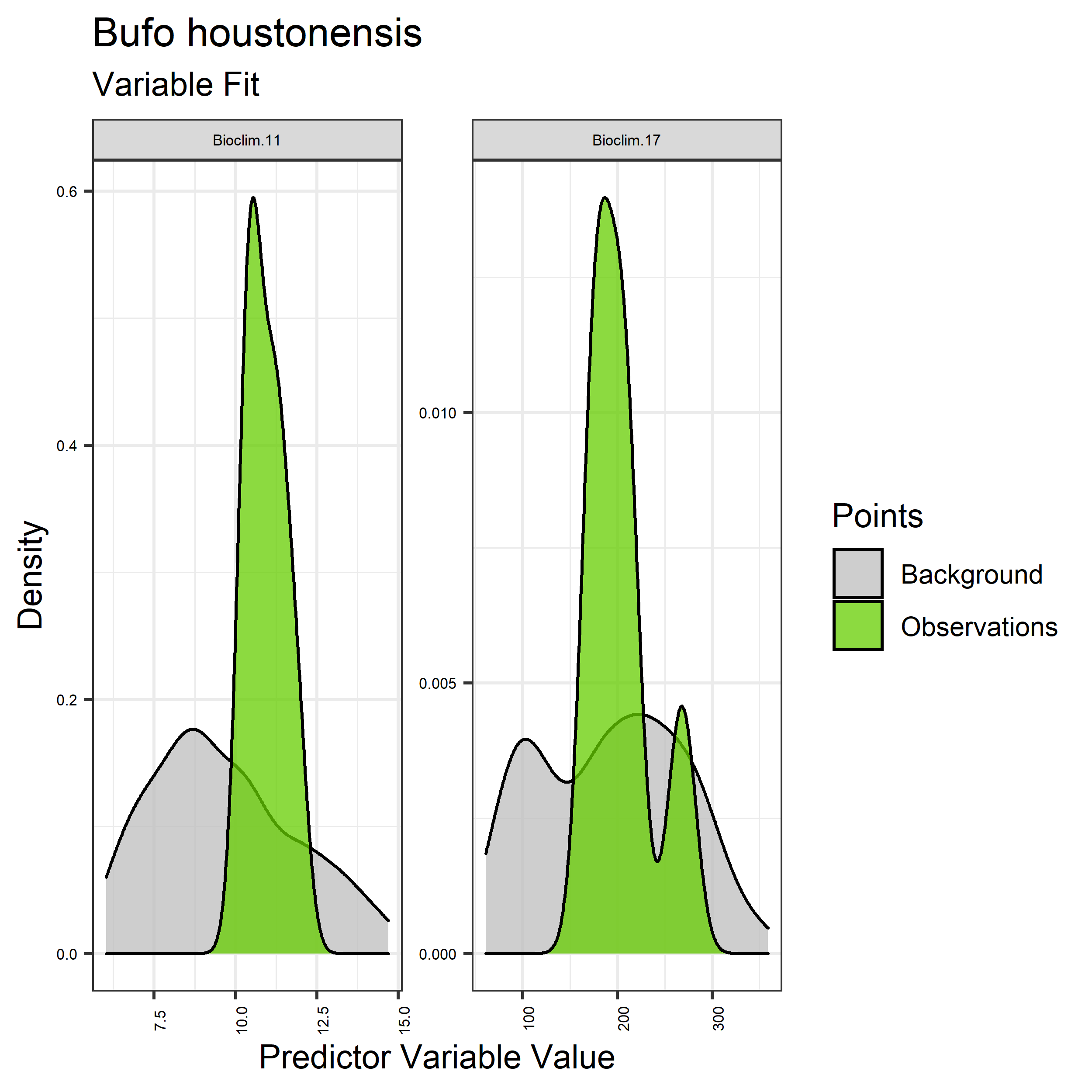
Figure 19. Sampling of continuous predictor variables retained in the best-fit Bufo houstonensis distribution models. Distribution of each variable at points of species occurrence (green) are contrasted with points sampled across the full modeled extent (gray).
|
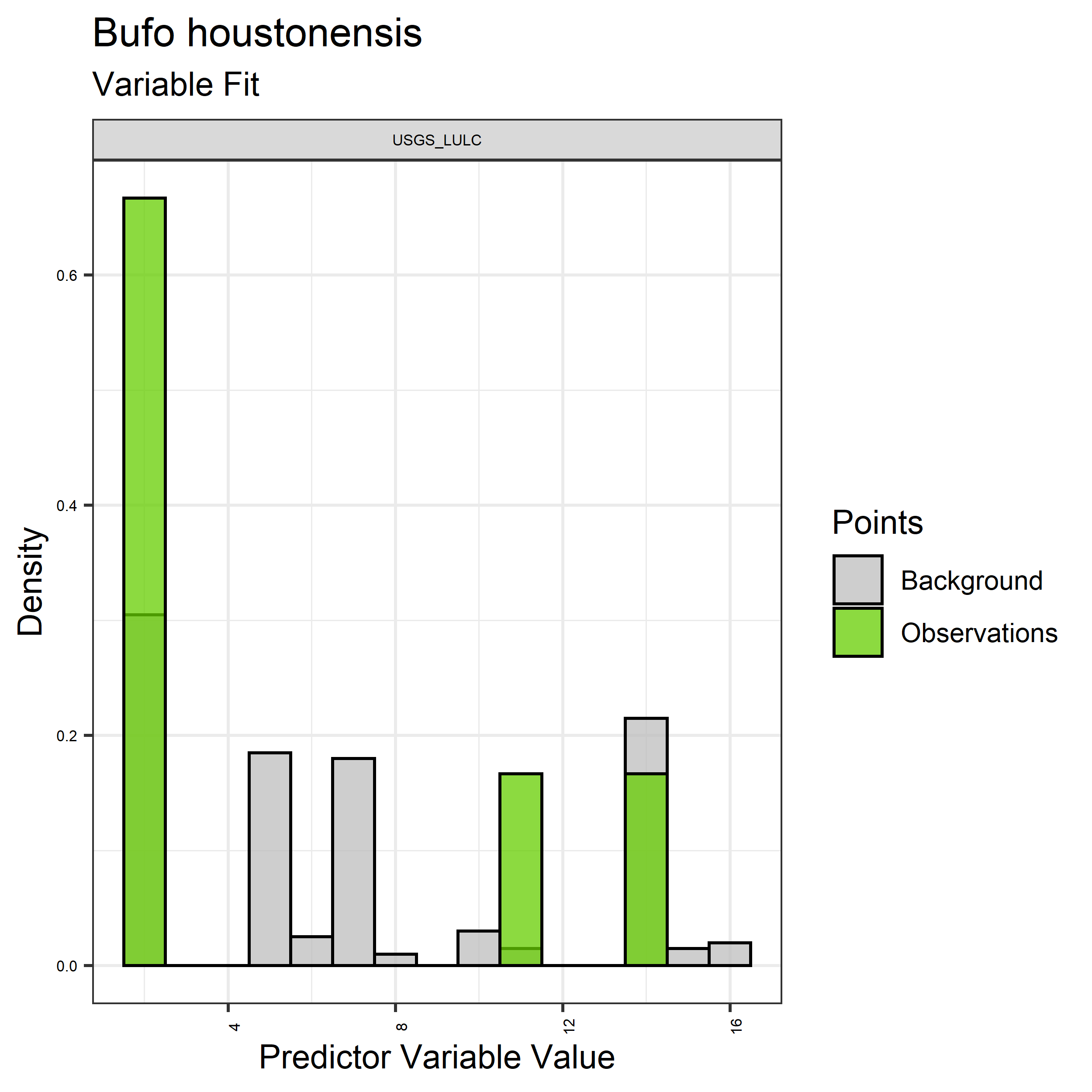
Figure 20. Sampling of discrete predictor variables retained in the best-fit Bufo houstonensis distribution models. Distribution of each variable at points of species occurrence (green) are contrasted with points sampled across the full modeled extent.
|
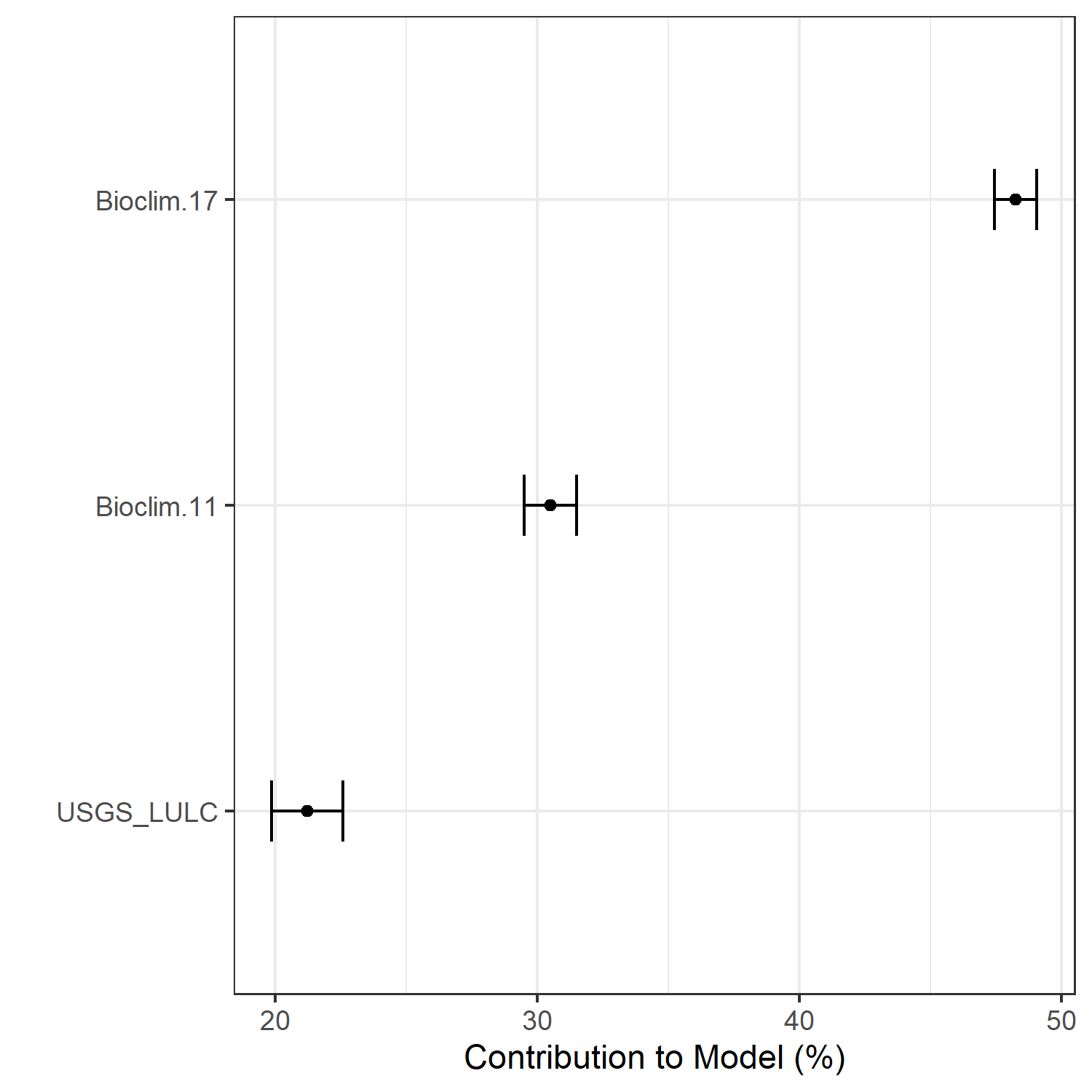
Figure 21. Percent contribution of each variable to best-fit species distribution models for Bufo houstonensis. Values sum to 1.0.
|
Table 12. Mean Area Under Curve (AUC) for five realizations of the best-fit SDM for Bufo houstonensis, calculated using 20% of species location records reserved for final evaluation.
| V1 |
V2 |
V3 |
V4 |
V5 |
mean |
sd |
| 0.921667 |
0.92 |
0.916667 |
0.923333 |
0.918333 |
0.92 |
0.002846 |
|
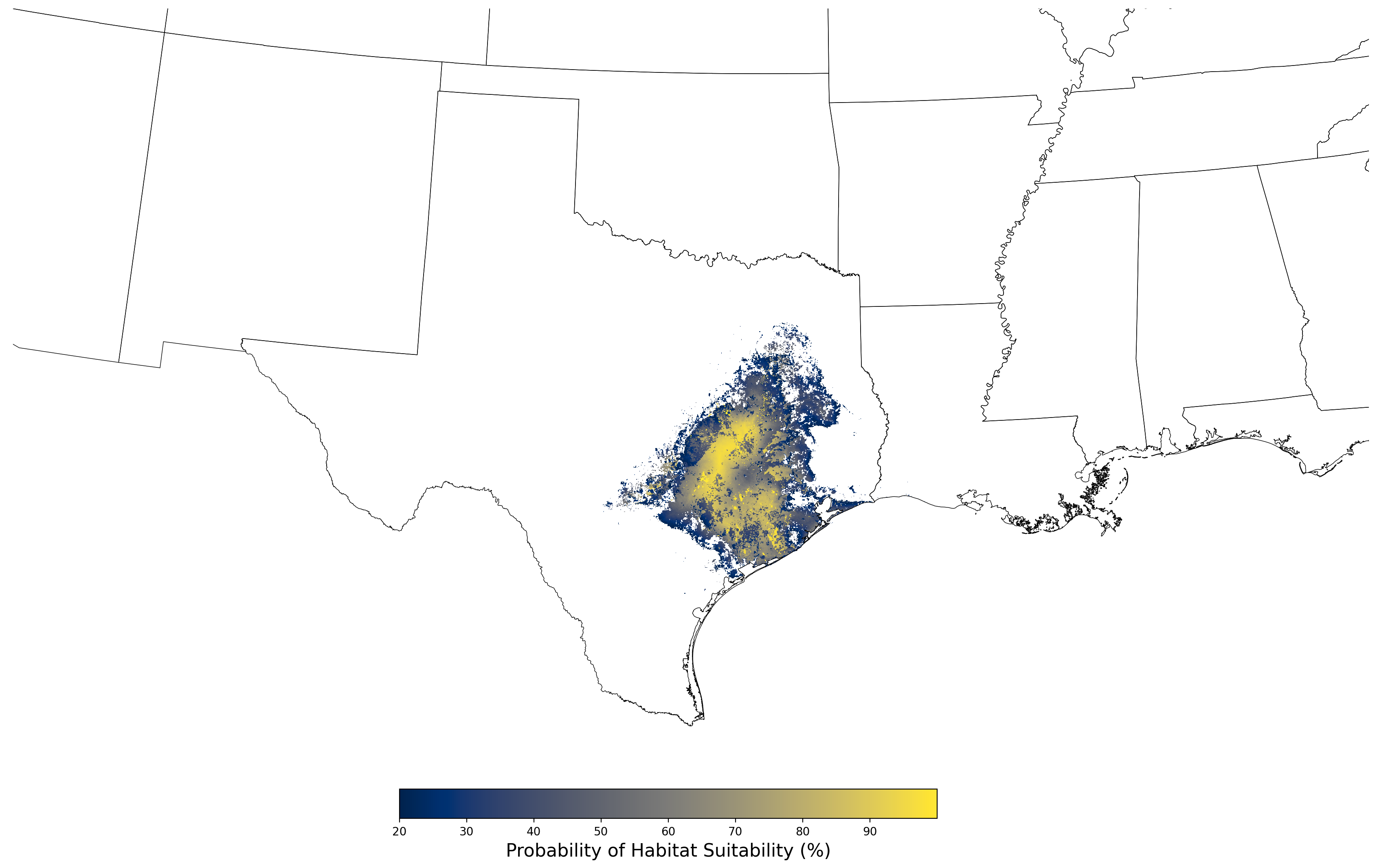
Figure 22. Final mean SDM output for Bufo houstonensis. |
2.2.4 Species Distribution Modeling Results for Chamaesyce garberi
The species distribution modeling results consist of the following figures and tables:
- A table showing the SDM inputs (Table 13)
- A map showing the extent of SDM coverage (Figure 23)
- A graph showing the correlation between the predictor variable selected for evaluation (Figure 24)
- A graph of the model fit of each SDM iteration as measured by total Area Under Curve (AUC) where the curve is the Receiver Operating Curve, based on training data (Figure 25)
- A table showing the diagnostic statistics of the training data used in the final selected SDM iteration (Table 14)
- Graphs illustrating the predictor variable values sampled by the species observations and randomly selected background locations for continuous variables (Figure 26), and discrete variables (Figure 27)
- A graph showing the percent contribution of each predictor variable to the final selected SDM (Figure 28)
- A table showing the mean AUC for each of the five model runs that are averaged for the final selected SDM (Table 15)
- A map of the final averaged SDM (Figure 29)
Table 13. Input parameters for species distribution modeling of Chamaesyce garberi.
| Number of predictors |
33 |
| Names of predictors |
Bioclim.01.tif, Bioclim.02.tif, Bioclim.03.tif, Bioclim.04.tif,
Bioclim.05.tif, Bioclim.06.tif, Bioclim.07.tif, Bioclim.08.tif,
Bioclim.09.tif, Bioclim.10.tif, Bioclim.11.tif, Bioclim.12.tif,
Bioclim.13.tif, Bioclim.14.tif, Bioclim.15.tif, Bioclim.16.tif,
Bioclim.17.tif, Bioclim.18.tif, Bioclim.19.tif, Elevation.tif,
Solar.APR.tif, Solar.AUG.tif, Solar.DEC.tif, Solar.FEB.tif,
Solar.JAN.tif, Solar.JUL.tif, Solar.JUN.tif, Solar.MAR.tif,
Solar.MAY.tif, Solar.NOV.tif, Solar.OCT.tif, Solar.SEP.tif,
USGS_LULC.tif |
| Predictor correlation threshold |
0.67 |
| Predictor contribution threshold |
1.0 |
| SDM threshold |
0.2 |
| Number of iterations conducted |
3 |
| Final SDM iteration number |
2 |
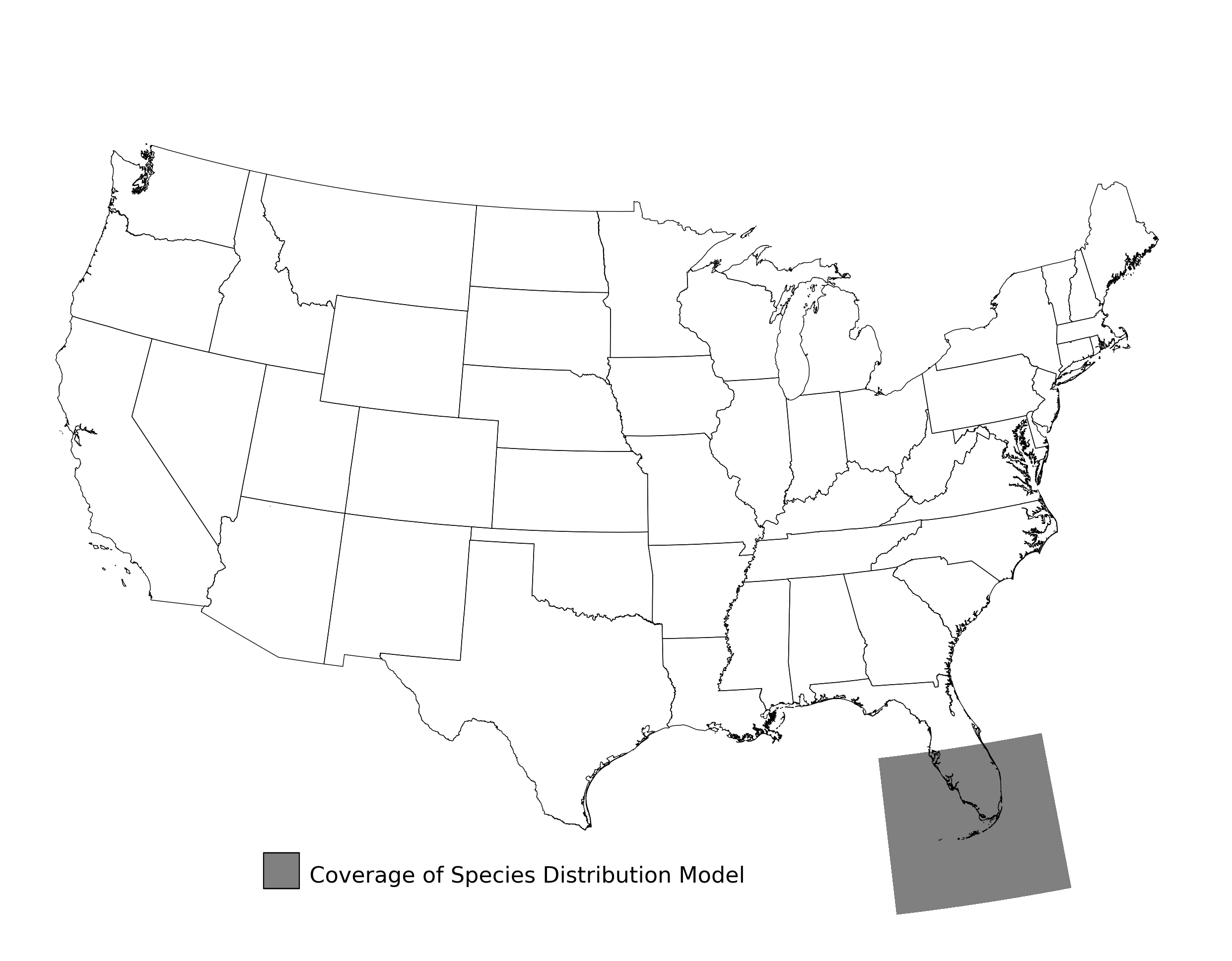
Figure 23. Extent of the species range modeled for Chamaesyce garberi. Modeling extent is determined by buffering species location records in all directions by 3 degrees latitude/longitude.
|
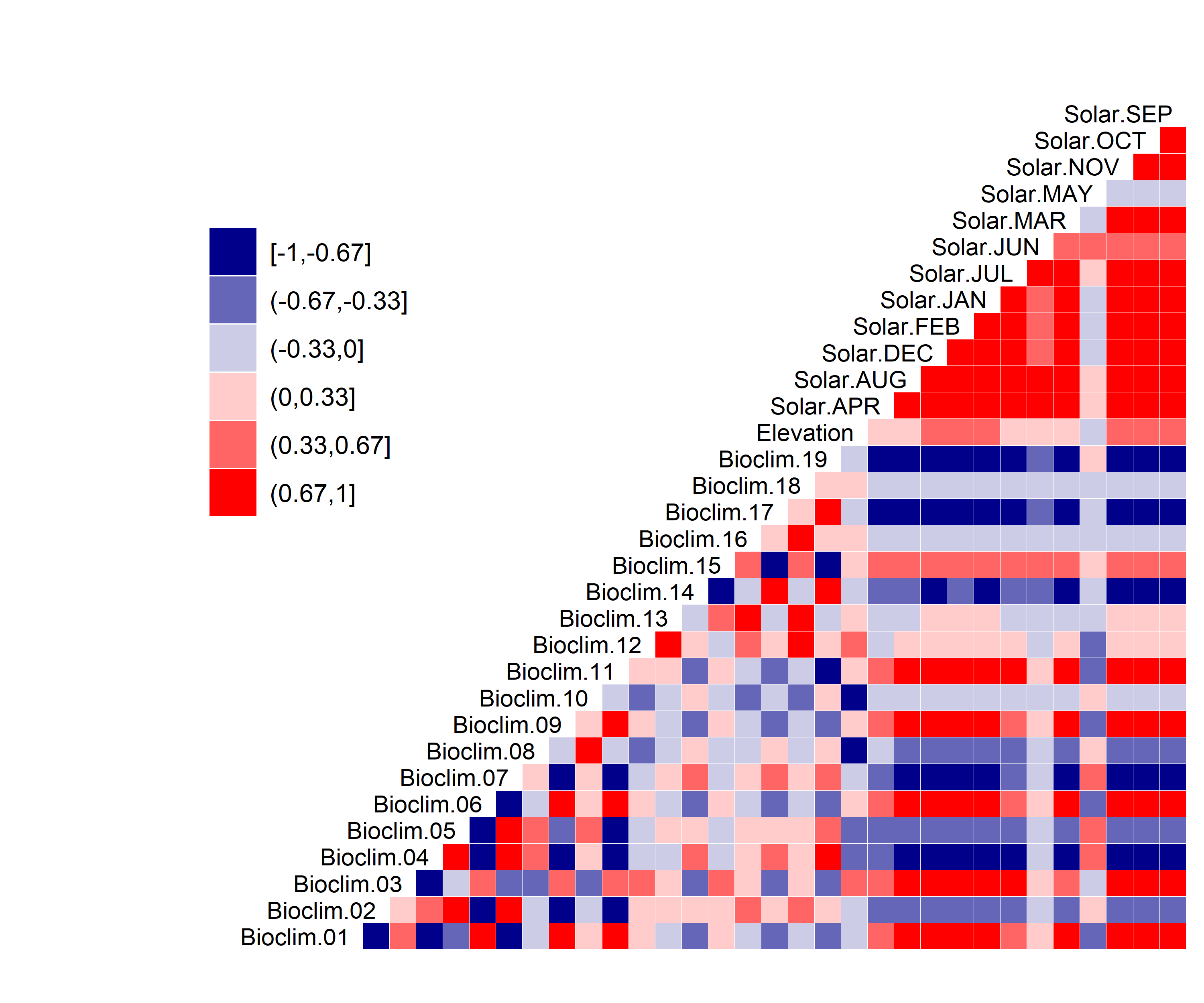
Figure 24. Correlation between SDM predictor variables for Chamaesyce garberi.
|
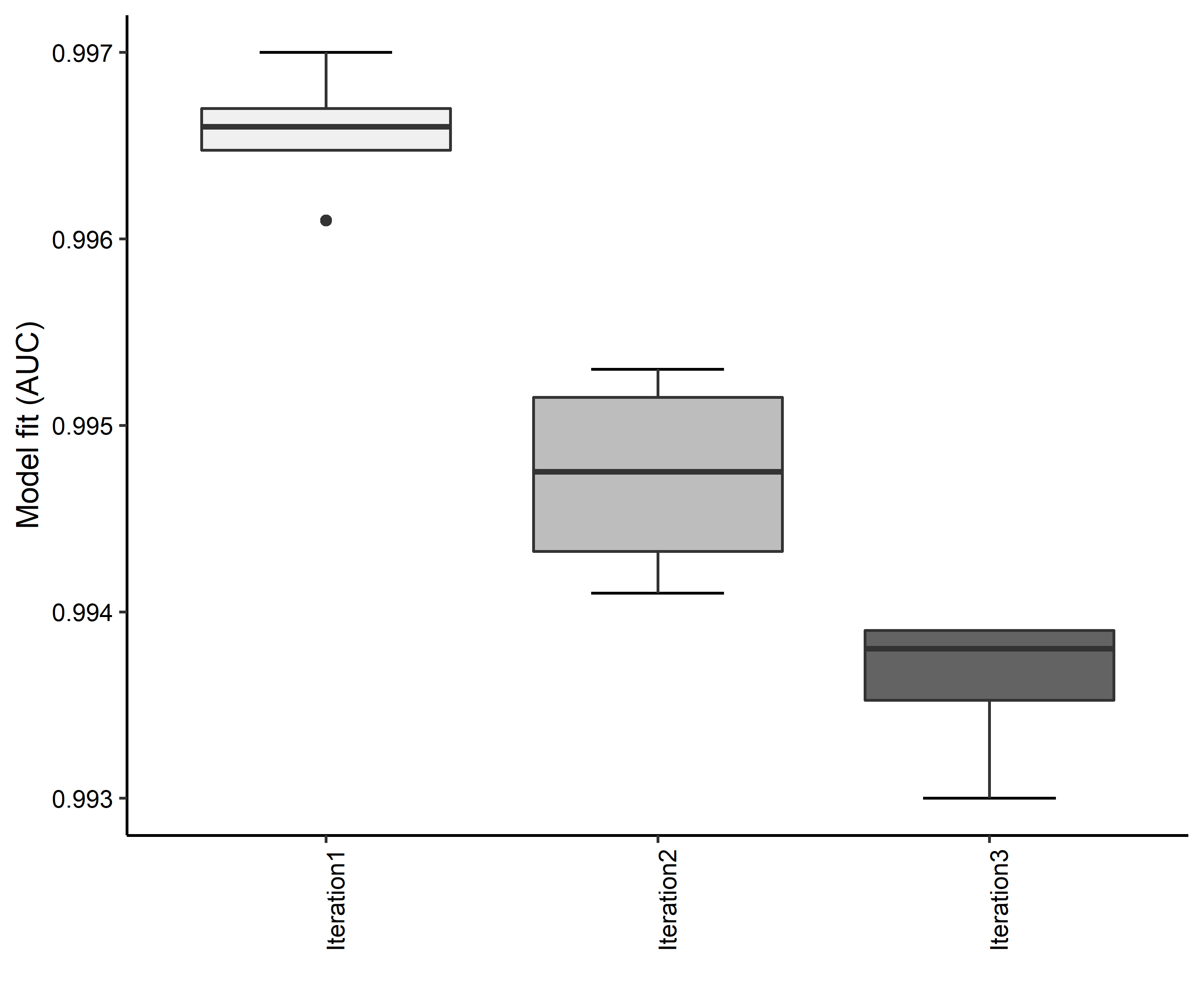
Figure 25. Boxplots of model fit for each iteration of Chamaesyce garberi distribution modeling. Statistics are calculated using 80% of species location records reserved for model training.
|
Table 14. Diagnostic statistics of the training data used in SDM iteration #2 for Chamaesyce garberi.
| Model Output |
Realization 1 |
Realization 2 |
Realization 3 |
Realization 4 |
Realization 5 |
Mean |
Standard Deviation |
| Number of training samples |
24.0000 |
24.0000 |
24.0000 |
24.0000 |
24.0000 |
24.00000 |
0.000000 |
| Regularized training gain |
3.7089 |
4.0232 |
3.7802 |
3.9350 |
3.8405 |
3.85756 |
0.124307 |
| Unregularized training gain |
4.2563 |
4.5495 |
4.2933 |
4.4887 |
4.3787 |
4.39330 |
0.124982 |
| Iterations |
500.0000 |
500.0000 |
500.0000 |
500.0000 |
500.0000 |
500.00000 |
0.000000 |
| Training AUC |
0.9942 |
0.9951 |
0.9941 |
0.9953 |
0.9944 |
0.99462 |
0.000545 |
| Number of background points |
10024.0000 |
10024.0000 |
10024.0000 |
10024.0000 |
10024.0000 |
10024.00000 |
0.000000 |
| Bioclim 02 contribution |
75.6359 |
72.1978 |
76.3608 |
78.4794 |
77.3784 |
76.01046 |
2.385704 |
| Bioclim 03 contribution |
12.1806 |
12.5614 |
8.8565 |
8.5005 |
8.6382 |
10.14744 |
2.038240 |
| Bioclim 13 contribution |
2.7805 |
0.6765 |
0.2338 |
2.9228 |
0.5371 |
1.43014 |
1.308456 |
| Bioclim 15 contribution |
4.3000 |
3.6890 |
2.4780 |
2.9671 |
2.4730 |
3.18142 |
0.798663 |
| Solar JUN contribution |
1.4270 |
5.5702 |
5.8307 |
1.3870 |
6.1065 |
4.06428 |
2.433196 |
| USGS_LULC contribution |
3.6760 |
5.3051 |
6.2401 |
5.7433 |
4.8668 |
5.16626 |
0.976721 |
| Bioclim 02 permutation importance |
51.3078 |
30.1871 |
48.1931 |
46.0461 |
48.1650 |
44.77982 |
8.370714 |
| Bioclim 03 permutation importance |
23.5929 |
40.1912 |
25.0939 |
34.5585 |
33.3547 |
31.35824 |
6.924434 |
| Bioclim 13 permutation importance |
0.3283 |
0.0000 |
0.0000 |
0.6659 |
0.1159 |
0.22202 |
0.282034 |
| Bioclim 15 permutation importance |
6.8977 |
4.0358 |
2.9589 |
3.8620 |
2.6365 |
4.07818 |
1.682963 |
| Solar JUN permutation importance |
13.3291 |
22.5150 |
19.6316 |
11.2105 |
11.8261 |
15.70246 |
5.066694 |
| USGS_LULC permutation importance |
4.5442 |
3.0709 |
4.1225 |
3.6569 |
3.9017 |
3.85924 |
0.548338 |
| Entropy |
5.5079 |
5.1900 |
5.4304 |
5.2799 |
5.3705 |
5.35574 |
0.124666 |
| Prevalence average probability of presence over background sites |
0.0125 |
0.0090 |
0.0115 |
0.0099 |
0.0108 |
0.01074 |
0.001361 |
| Fixed cumulative value 1 cumulative threshold |
1.0000 |
1.0000 |
1.0000 |
1.0000 |
1.0000 |
1.00000 |
0.000000 |
| Fixed cumulative value 1 Cloglog threshold |
0.0019 |
0.0014 |
0.0018 |
0.0016 |
0.0017 |
0.00168 |
0.000192 |
| Fixed cumulative value 1 area |
0.2772 |
0.2533 |
0.2676 |
0.2573 |
0.2687 |
0.26482 |
0.009557 |
| Fixed cumulative value 1 training omission |
0.0000 |
0.0000 |
0.0000 |
0.0000 |
0.0000 |
0.00000 |
0.000000 |
| Fixed cumulative value 5 cumulative threshold |
5.0000 |
5.0000 |
5.0000 |
5.0000 |
5.0000 |
5.00000 |
0.000000 |
| Fixed cumulative value 5 Cloglog threshold |
0.0122 |
0.0097 |
0.0111 |
0.0099 |
0.0102 |
0.01062 |
0.001033 |
| Fixed cumulative value 5 area |
0.0939 |
0.0762 |
0.0896 |
0.0813 |
0.0901 |
0.08622 |
0.007247 |
| Fixed cumulative value 5 training omission |
0.0000 |
0.0000 |
0.0000 |
0.0000 |
0.0000 |
0.00000 |
0.000000 |
| Fixed cumulative value 10 cumulative threshold |
10.0000 |
10.0000 |
10.0000 |
10.0000 |
10.0000 |
10.00000 |
0.000000 |
| Fixed cumulative value 10 Cloglog threshold |
0.0433 |
0.0386 |
0.0424 |
0.0406 |
0.0385 |
0.04068 |
0.002174 |
| Fixed cumulative value 10 area |
0.0377 |
0.0299 |
0.0353 |
0.0306 |
0.0333 |
0.03336 |
0.003248 |
| Fixed cumulative value 10 training omission |
0.0417 |
0.0417 |
0.0417 |
0.0417 |
0.0417 |
0.04170 |
0.000000 |
| Minimum training presence cumulative threshold |
7.7649 |
6.4834 |
6.6934 |
7.9143 |
6.9917 |
7.16954 |
0.639970 |
| Minimum training presence Cloglog threshold |
0.0250 |
0.0159 |
0.0185 |
0.0240 |
0.0177 |
0.02022 |
0.004034 |
| Minimum training presence area |
0.0544 |
0.0544 |
0.0621 |
0.0436 |
0.0583 |
0.05456 |
0.006910 |
| Minimum training presence training omission |
0.0000 |
0.0000 |
0.0000 |
0.0000 |
0.0000 |
0.00000 |
0.000000 |
| X10 percentile training presence cumulative threshold |
21.6029 |
19.0153 |
22.3198 |
20.6189 |
21.9350 |
21.09838 |
1.324336 |
| X10 percentile training presence Cloglog threshold |
0.2521 |
0.1773 |
0.2904 |
0.2371 |
0.2971 |
0.25080 |
0.048227 |
| X10 percentile training presence area |
0.0115 |
0.0106 |
0.0098 |
0.0091 |
0.0094 |
0.01008 |
0.000973 |
| X10 percentile training presence training omission |
0.0833 |
0.0833 |
0.0833 |
0.0833 |
0.0833 |
0.08330 |
0.000000 |
| Equal training sensitivity and specificity cumulative threshold |
9.3439 |
7.9101 |
8.9345 |
8.1685 |
8.7174 |
8.61488 |
0.578815 |
| Equal training sensitivity and specificity Cloglog threshold |
0.0368 |
0.0253 |
0.0333 |
0.0252 |
0.0285 |
0.02982 |
0.005108 |
| Equal training sensitivity and specificity area |
0.0417 |
0.0417 |
0.0417 |
0.0417 |
0.0417 |
0.04170 |
0.000000 |
| Equal training sensitivity and specificity training omission |
0.0417 |
0.0417 |
0.0417 |
0.0417 |
0.0417 |
0.04170 |
0.000000 |
| Maximum training sensitivity plus specificity cumulative threshold |
7.7649 |
18.1811 |
18.5131 |
7.9143 |
15.9971 |
13.67410 |
5.413392 |
| Maximum training sensitivity plus specificity Cloglog threshold |
0.0250 |
0.1615 |
0.1693 |
0.0240 |
0.1247 |
0.10090 |
0.071749 |
| Maximum training sensitivity plus specificity area |
0.0544 |
0.0114 |
0.0132 |
0.0436 |
0.0154 |
0.02760 |
0.019955 |
| Maximum training sensitivity plus specificity training omission |
0.0000 |
0.0417 |
0.0417 |
0.0000 |
0.0417 |
0.02502 |
0.022840 |
| Balance training omission predicted area and threshold value cumulative threshold |
4.1836 |
4.0525 |
4.1698 |
4.1412 |
4.2704 |
4.16350 |
0.078565 |
| Balance training omission predicted area and threshold value Cloglog threshold |
0.0098 |
0.0071 |
0.0091 |
0.0078 |
0.0085 |
0.00846 |
0.001060 |
| Balance training omission predicted area and threshold value area |
0.1122 |
0.0967 |
0.1085 |
0.1006 |
0.1068 |
0.10496 |
0.006236 |
| Balance training omission predicted area and threshold value training omission |
0.0000 |
0.0000 |
0.0000 |
0.0000 |
0.0000 |
0.00000 |
0.000000 |
| Equate entropy of thresholded and original distributions cumulative threshold |
13.2955 |
13.8466 |
13.3086 |
13.1406 |
13.1486 |
13.34798 |
0.289692 |
| Equate entropy of thresholded and original distributions Cloglog threshold |
0.0833 |
0.0807 |
0.0791 |
0.0753 |
0.0742 |
0.07852 |
0.003774 |
| Equate entropy of thresholded and original distributions area |
0.0245 |
0.0179 |
0.0227 |
0.0196 |
0.0213 |
0.02120 |
0.002579 |
| Equate entropy of thresholded and original distributions training omission |
0.0417 |
0.0417 |
0.0417 |
0.0417 |
0.0417 |
0.04170 |
0.000000 |
|
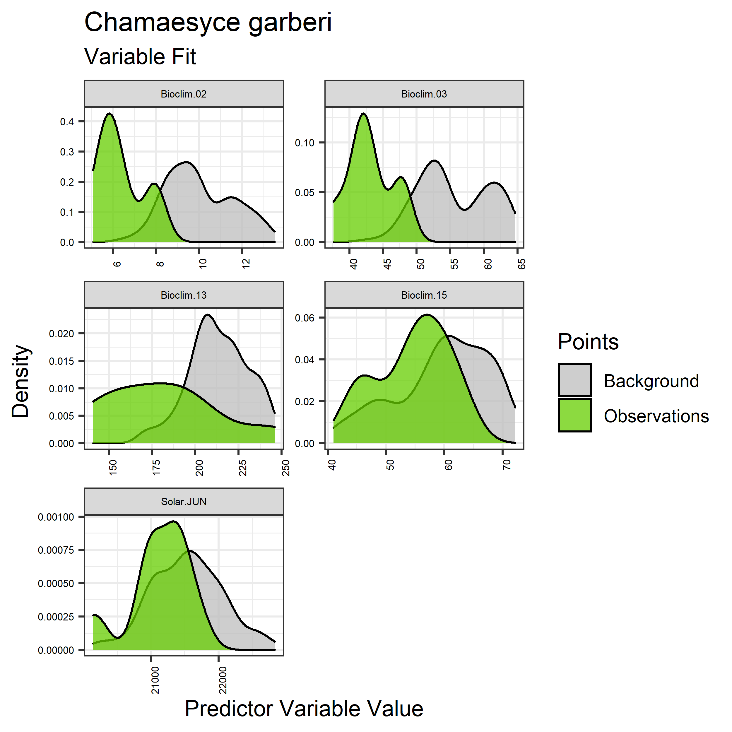
Figure 26. Sampling of continuous predictor variables retained in the best-fit Chamaesyce garberi distribution models. Distribution of each variable at points of species occurrence (green) are contrasted with points sampled across the full modeled extent (gray).
|
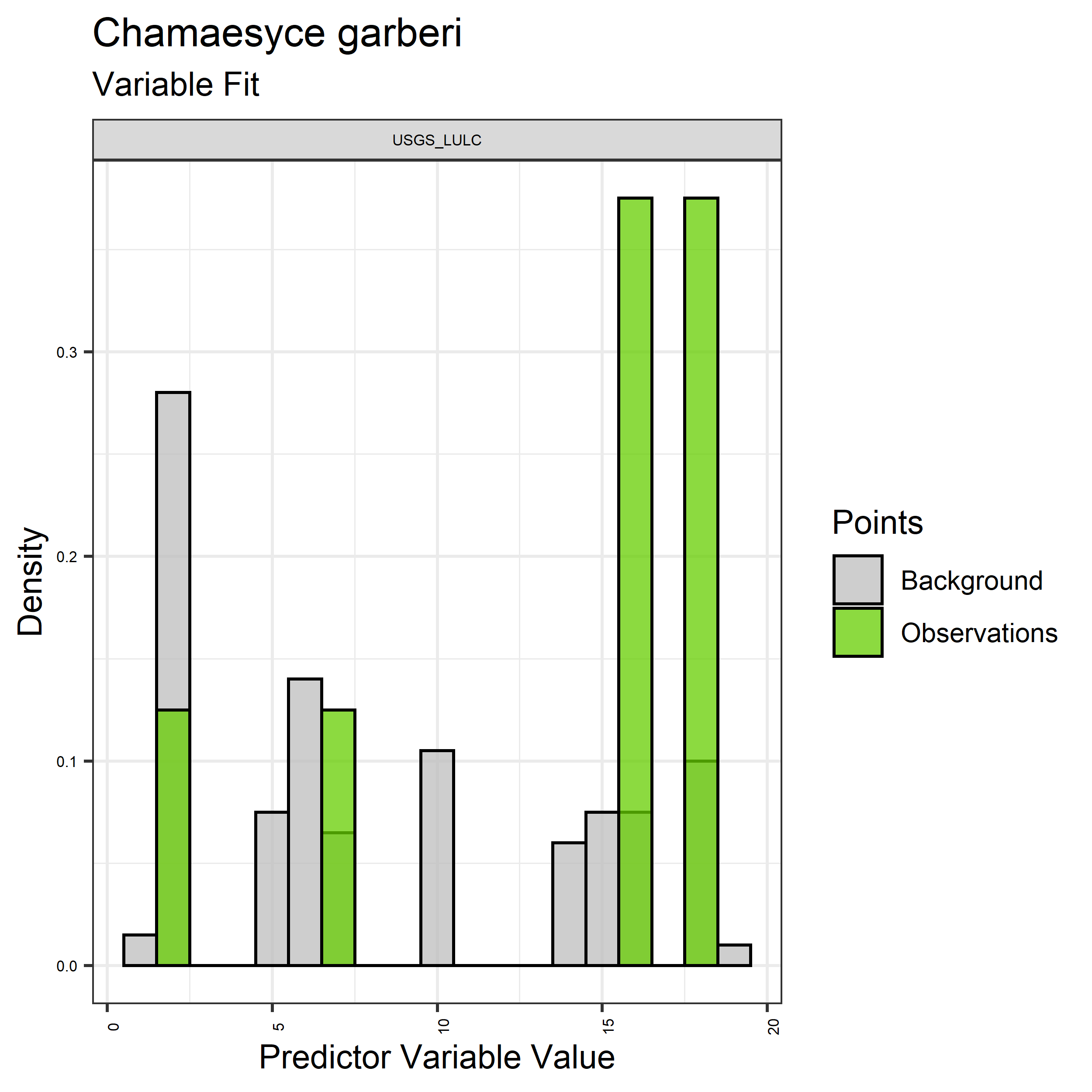
Figure 27. Sampling of discrete predictor variables retained in the best-fit Chamaesyce garberi distribution models. Distribution of each variable at points of species occurrence (green) are contrasted with points sampled across the full modeled extent.
|
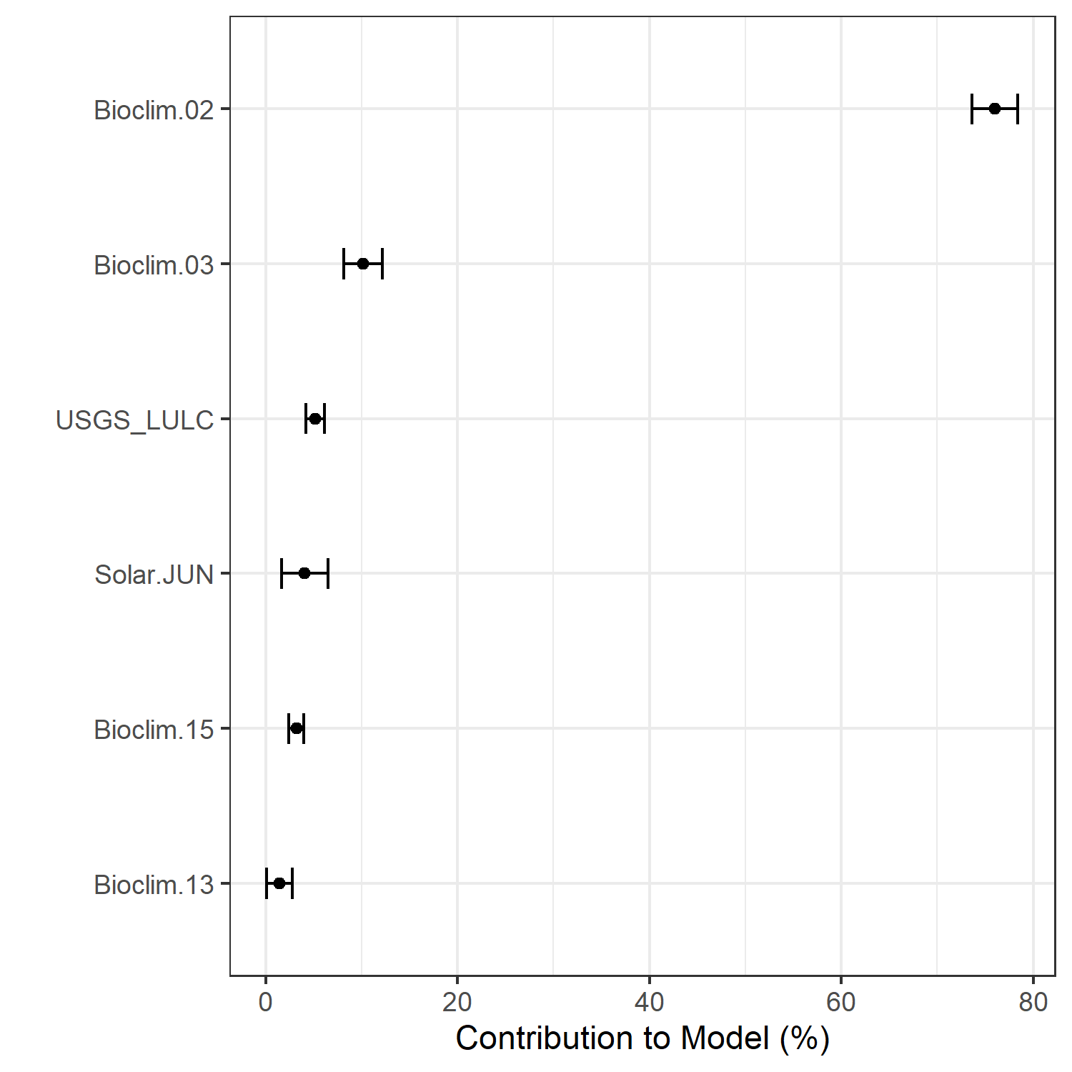
Figure 28. Percent contribution of each variable to best-fit species distribution models for Chamaesyce garberi. Values sum to 1.0.
|
Table 15. Mean Area Under Curve (AUC) for five realizations of the best-fit SDM for Chamaesyce garberi, calculated using 20% of species location records reserved for final evaluation.
| V1 |
V2 |
V3 |
V4 |
V5 |
mean |
sd |
| 0.996875 |
0.995625 |
0.99625 |
0.99625 |
0.99625 |
0.99625 |
0 |
|
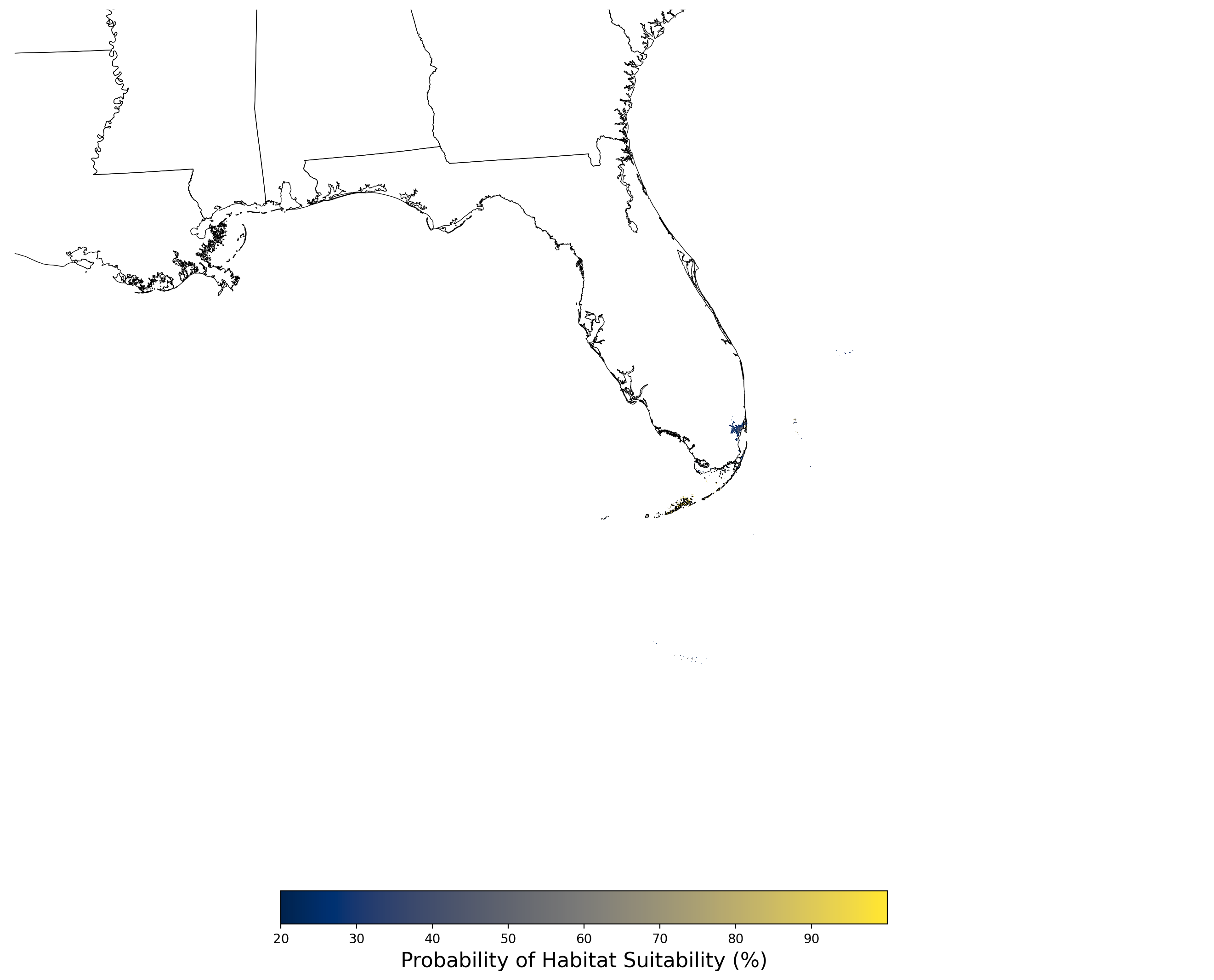
Figure 29. Final mean SDM output for Chamaesyce garberi. |
2.2.5 Species Distribution Modeling Results for Cicindela puritana
The species distribution modeling results consist of the following figures and tables:
- A table showing the SDM inputs (Table 16)
- A map showing the extent of SDM coverage (Figure 30)
- A graph showing the correlation between the predictor variable selected for evaluation (Figure 31)
- A graph of the model fit of each SDM iteration as measured by total Area Under Curve (AUC) where the curve is the Receiver Operating Curve, based on training data (Figure 32)
- A table showing the diagnostic statistics of the training data used in the final selected SDM iteration (Table 17)
- Graphs illustrating the predictor variable values sampled by the species observations and randomly selected background locations for continuous variables (Figure 33), and discrete variables (Figure 34)
- A graph showing the percent contribution of each predictor variable to the final selected SDM (Figure 35)
- A table showing the mean AUC for each of the five model runs that are averaged for the final selected SDM (Table 18)
- A map of the final averaged SDM (Figure 36)
Table 16. Input parameters for species distribution modeling of Bombus affinis.
| Number of predictors |
33 |
| Names of predictors |
Bioclim.01.tif, Bioclim.02.tif, Bioclim.03.tif, Bioclim.04.tif,
Bioclim.05.tif, Bioclim.06.tif, Bioclim.07.tif, Bioclim.08.tif,
Bioclim.09.tif, Bioclim.10.tif, Bioclim.11.tif, Bioclim.12.tif,
Bioclim.13.tif, Bioclim.14.tif, Bioclim.15.tif, Bioclim.16.tif,
Bioclim.17.tif, Bioclim.18.tif, Bioclim.19.tif, Elevation.tif,
Solar.APR.tif, Solar.AUG.tif, Solar.DEC.tif, Solar.FEB.tif,
Solar.JAN.tif, Solar.JUL.tif, Solar.JUN.tif, Solar.MAR.tif,
Solar.MAY.tif, Solar.NOV.tif, Solar.OCT.tif, Solar.SEP.tif,
USGS_LULC.tif |
| Predictor correlation threshold |
0.67 |
| Predictor contribution threshold |
1.0 |
| SDM threshold |
0.2 |
| Number of iterations conducted |
3 |
| Final SDM iteration number |
2 |
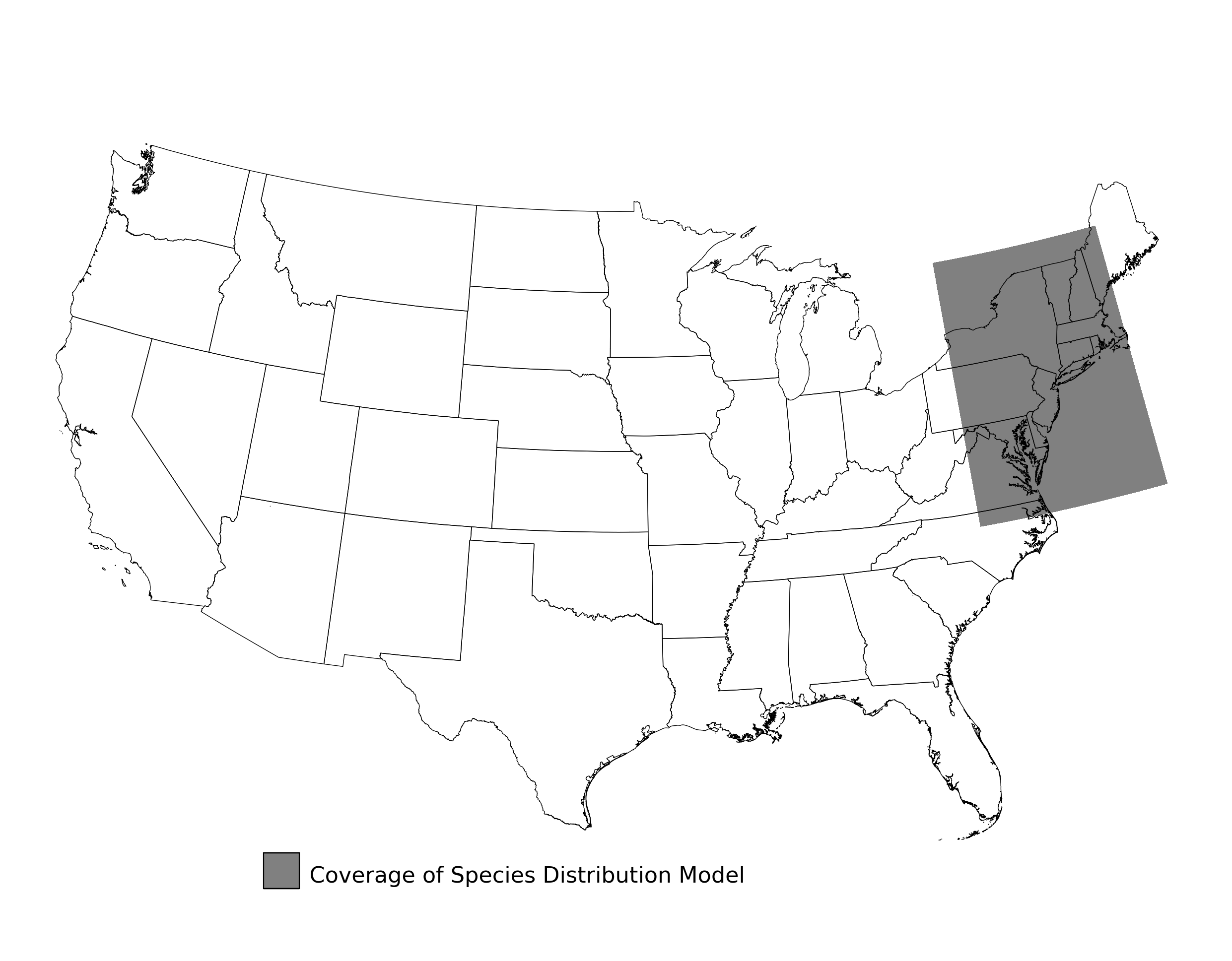
Figure 30. Extent of the species range modeled for Cicindela puritana. Modeling extent is determined by buffering species location records in all directions by 3 degrees latitude/longitude.
|
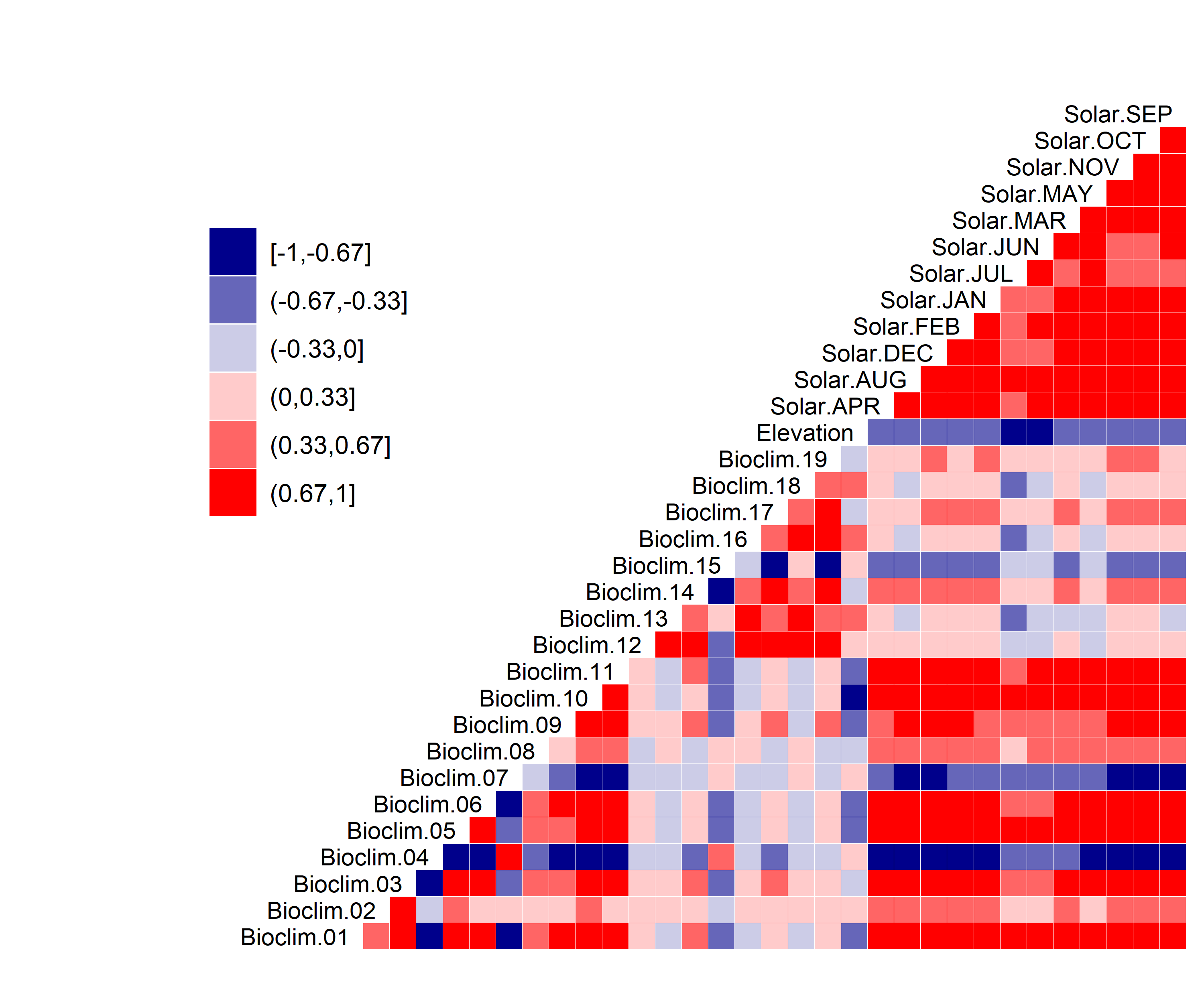
Figure 31. Correlation between SDM predictor variables for Cicindela puritana.
|
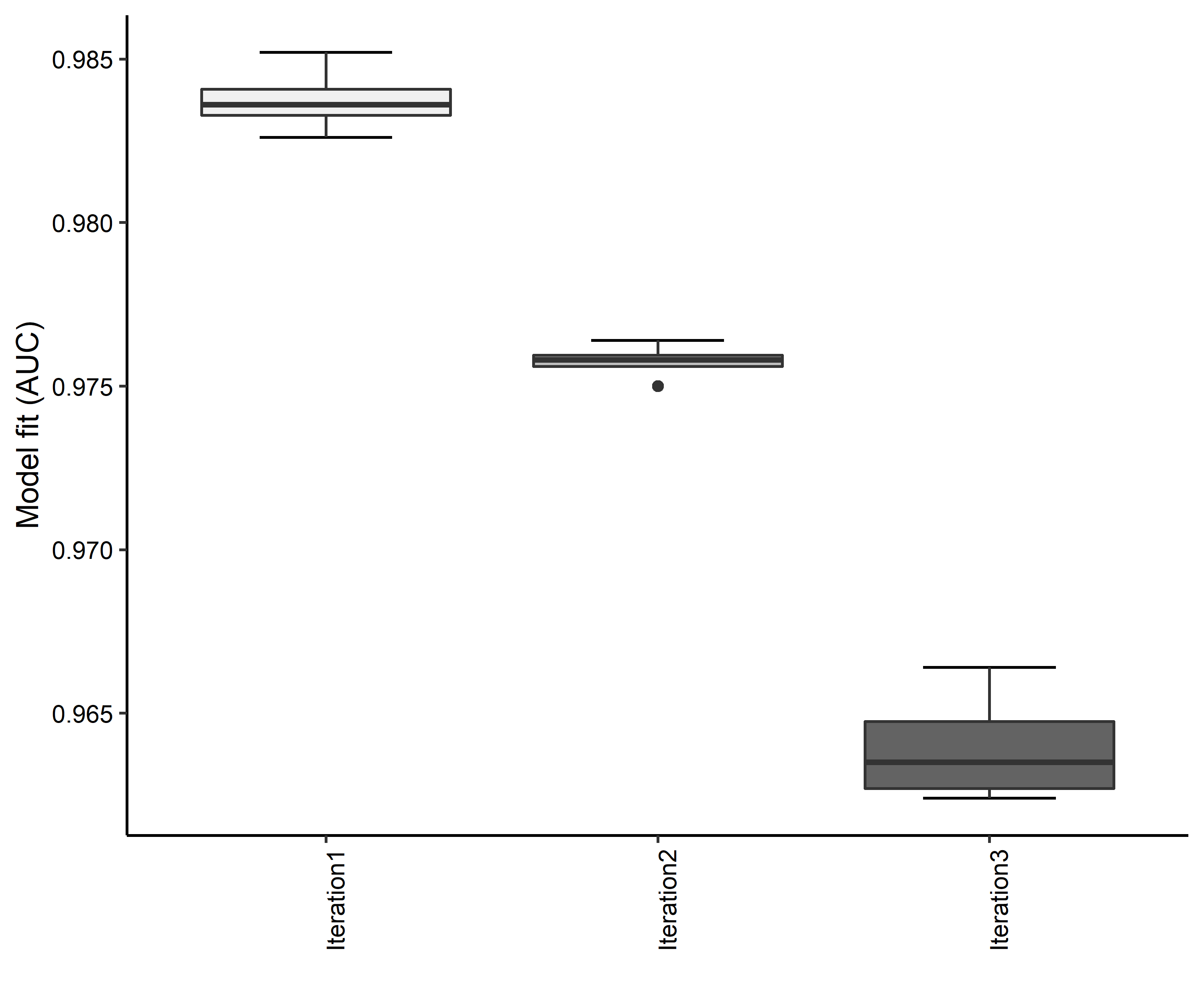
Figure 32. Boxplots of model fit for each iteration of Cicindela puritana distribution modeling. Statistics are calculated using 80% of species location records reserved for model training.
|
Table 17. Diagnostic statistics of the training data used in SDM iteration #2 for Cicindela puritana.
| Model Output |
Realization 1 |
Realization 2 |
Realization 3 |
Realization 4 |
Realization 5 |
Mean |
Standard Deviation |
| Number of training samples |
14.0000 |
14.0000 |
14.0000 |
14.0000 |
14.0000 |
14.00000 |
0.000000 |
| Regularized training gain |
2.2708 |
2.2461 |
2.3297 |
2.2305 |
2.2227 |
2.25996 |
0.043097 |
| Unregularized training gain |
2.7060 |
2.6700 |
2.7845 |
2.6583 |
2.6741 |
2.69858 |
0.051176 |
| Iterations |
200.0000 |
200.0000 |
160.0000 |
160.0000 |
240.0000 |
192.00000 |
33.466401 |
| Training AUC |
0.9762 |
0.9750 |
0.9764 |
0.9758 |
0.9758 |
0.97584 |
0.000537 |
| Number of background points |
10014.0000 |
10014.0000 |
10014.0000 |
10014.0000 |
10014.0000 |
10014.00000 |
0.000000 |
| Bioclim 13 contribution |
8.3690 |
7.5021 |
9.3327 |
8.0313 |
7.8574 |
8.21850 |
0.696914 |
| Bioclim 15 contribution |
18.4082 |
19.7338 |
17.5497 |
17.8592 |
19.1371 |
18.53760 |
0.900446 |
| Elevation contribution |
37.8710 |
34.1192 |
46.2148 |
40.0823 |
34.9763 |
38.65272 |
4.845325 |
| Solar OCT contribution |
14.7525 |
17.1882 |
9.1908 |
14.1645 |
16.8798 |
14.43516 |
3.210637 |
| USGS_LULC contribution |
20.5993 |
21.4566 |
17.7119 |
19.8628 |
21.1494 |
20.15600 |
1.494533 |
| Bioclim 13 permutation importance |
7.8572 |
9.2356 |
6.6306 |
7.5954 |
8.3382 |
7.93140 |
0.958763 |
| Bioclim 15 permutation importance |
28.2208 |
8.6538 |
22.9939 |
20.1363 |
22.1875 |
20.43846 |
7.230556 |
| Elevation permutation importance |
61.9849 |
79.0694 |
65.7468 |
68.6667 |
67.6599 |
68.62554 |
6.371688 |
| Solar OCT permutation importance |
0.7654 |
0.6686 |
1.1132 |
0.7953 |
0.8315 |
0.83480 |
0.166970 |
| USGS_LULC permutation importance |
1.1718 |
2.3726 |
3.5155 |
2.8064 |
0.9830 |
2.16986 |
1.079559 |
| Entropy |
6.9410 |
6.9656 |
6.8819 |
6.9813 |
6.9892 |
6.95180 |
0.043192 |
| Prevalence average probability of presence over background sites |
0.0583 |
0.0605 |
0.0552 |
0.0610 |
0.0615 |
0.05930 |
0.002597 |
| Fixed cumulative value 1 cumulative threshold |
1.0000 |
1.0000 |
1.0000 |
1.0000 |
1.0000 |
1.00000 |
0.000000 |
| Fixed cumulative value 1 Cloglog threshold |
0.0157 |
0.0162 |
0.0154 |
0.0162 |
0.0180 |
0.01630 |
0.001010 |
| Fixed cumulative value 1 area |
0.2864 |
0.2882 |
0.2768 |
0.2869 |
0.2816 |
0.28398 |
0.004728 |
| Fixed cumulative value 1 training omission |
0.0000 |
0.0000 |
0.0000 |
0.0000 |
0.0000 |
0.00000 |
0.000000 |
| Fixed cumulative value 5 cumulative threshold |
5.0000 |
5.0000 |
5.0000 |
5.0000 |
5.0000 |
5.00000 |
0.000000 |
| Fixed cumulative value 5 Cloglog threshold |
0.0706 |
0.0735 |
0.0697 |
0.0744 |
0.0752 |
0.07268 |
0.002408 |
| Fixed cumulative value 5 area |
0.1761 |
0.1812 |
0.1747 |
0.1814 |
0.1791 |
0.17850 |
0.003011 |
| Fixed cumulative value 5 training omission |
0.0000 |
0.0000 |
0.0000 |
0.0000 |
0.0000 |
0.00000 |
0.000000 |
| Fixed cumulative value 10 cumulative threshold |
10.0000 |
10.0000 |
10.0000 |
10.0000 |
10.0000 |
10.00000 |
0.000000 |
| Fixed cumulative value 10 Cloglog threshold |
0.1319 |
0.1393 |
0.1264 |
0.1360 |
0.1372 |
0.13416 |
0.005108 |
| Fixed cumulative value 10 area |
0.1274 |
0.1320 |
0.1260 |
0.1315 |
0.1302 |
0.12942 |
0.002616 |
| Fixed cumulative value 10 training omission |
0.0000 |
0.0000 |
0.0000 |
0.0000 |
0.0000 |
0.00000 |
0.000000 |
| Minimum training presence cumulative threshold |
14.4581 |
12.7686 |
12.3067 |
14.9498 |
15.2998 |
13.95660 |
1.339370 |
| Minimum training presence Cloglog threshold |
0.1815 |
0.1723 |
0.1491 |
0.1891 |
0.1962 |
0.17764 |
0.018260 |
| Minimum training presence area |
0.1001 |
0.1146 |
0.1108 |
0.1012 |
0.0984 |
0.10502 |
0.007208 |
| Minimum training presence training omission |
0.0000 |
0.0000 |
0.0000 |
0.0000 |
0.0000 |
0.00000 |
0.000000 |
| X10 percentile training presence cumulative threshold |
21.6107 |
24.2630 |
21.4414 |
20.5209 |
20.2773 |
21.62266 |
1.583372 |
| X10 percentile training presence Cloglog threshold |
0.2608 |
0.2995 |
0.2494 |
0.2587 |
0.2648 |
0.26664 |
0.019219 |
| X10 percentile training presence area |
0.0704 |
0.0671 |
0.0700 |
0.0770 |
0.0774 |
0.07238 |
0.004583 |
| X10 percentile training presence training omission |
0.0714 |
0.0714 |
0.0714 |
0.0714 |
0.0714 |
0.07140 |
0.000000 |
| Equal training sensitivity and specificity cumulative threshold |
21.3489 |
22.8871 |
21.0319 |
20.5209 |
20.2773 |
21.21322 |
1.025721 |
| Equal training sensitivity and specificity Cloglog threshold |
0.2586 |
0.2776 |
0.2457 |
0.2587 |
0.2648 |
0.26108 |
0.011566 |
| Equal training sensitivity and specificity area |
0.0714 |
0.0714 |
0.0714 |
0.0770 |
0.0774 |
0.07372 |
0.003180 |
| Equal training sensitivity and specificity training omission |
0.0714 |
0.0714 |
0.0714 |
0.0714 |
0.0714 |
0.07140 |
0.000000 |
| Maximum training sensitivity plus specificity cumulative threshold |
14.4581 |
12.7686 |
12.3067 |
14.9498 |
15.2998 |
13.95660 |
1.339370 |
| Maximum training sensitivity plus specificity Cloglog threshold |
0.1815 |
0.1723 |
0.1491 |
0.1891 |
0.1962 |
0.17764 |
0.018260 |
| Maximum training sensitivity plus specificity area |
0.1001 |
0.1146 |
0.1108 |
0.1012 |
0.0984 |
0.10502 |
0.007208 |
| Maximum training sensitivity plus specificity training omission |
0.0000 |
0.0000 |
0.0000 |
0.0000 |
0.0000 |
0.00000 |
0.000000 |
| Balance training omission predicted area and threshold value cumulative threshold |
2.7718 |
2.6689 |
2.5058 |
2.6335 |
2.5404 |
2.62408 |
0.105961 |
| Balance training omission predicted area and threshold value Cloglog threshold |
0.0404 |
0.0414 |
0.0382 |
0.0420 |
0.0422 |
0.04084 |
0.001633 |
| Balance training omission predicted area and threshold value area |
0.2173 |
0.2238 |
0.2201 |
0.2247 |
0.2242 |
0.22202 |
0.003204 |
| Balance training omission predicted area and threshold value training omission |
0.0000 |
0.0000 |
0.0000 |
0.0000 |
0.0000 |
0.00000 |
0.000000 |
| Equate entropy of thresholded and original distributions cumulative threshold |
13.8875 |
14.4479 |
14.7771 |
13.7814 |
13.4360 |
14.06598 |
0.538811 |
| Equate entropy of thresholded and original distributions Cloglog threshold |
0.1759 |
0.1894 |
0.1760 |
0.1743 |
0.1754 |
0.17820 |
0.006297 |
| Equate entropy of thresholded and original distributions area |
0.1032 |
0.1058 |
0.0973 |
0.1074 |
0.1082 |
0.10438 |
0.004395 |
| Equate entropy of thresholded and original distributions training omission |
0.0000 |
0.0714 |
0.0714 |
0.0000 |
0.0000 |
0.02856 |
0.039107 |
|
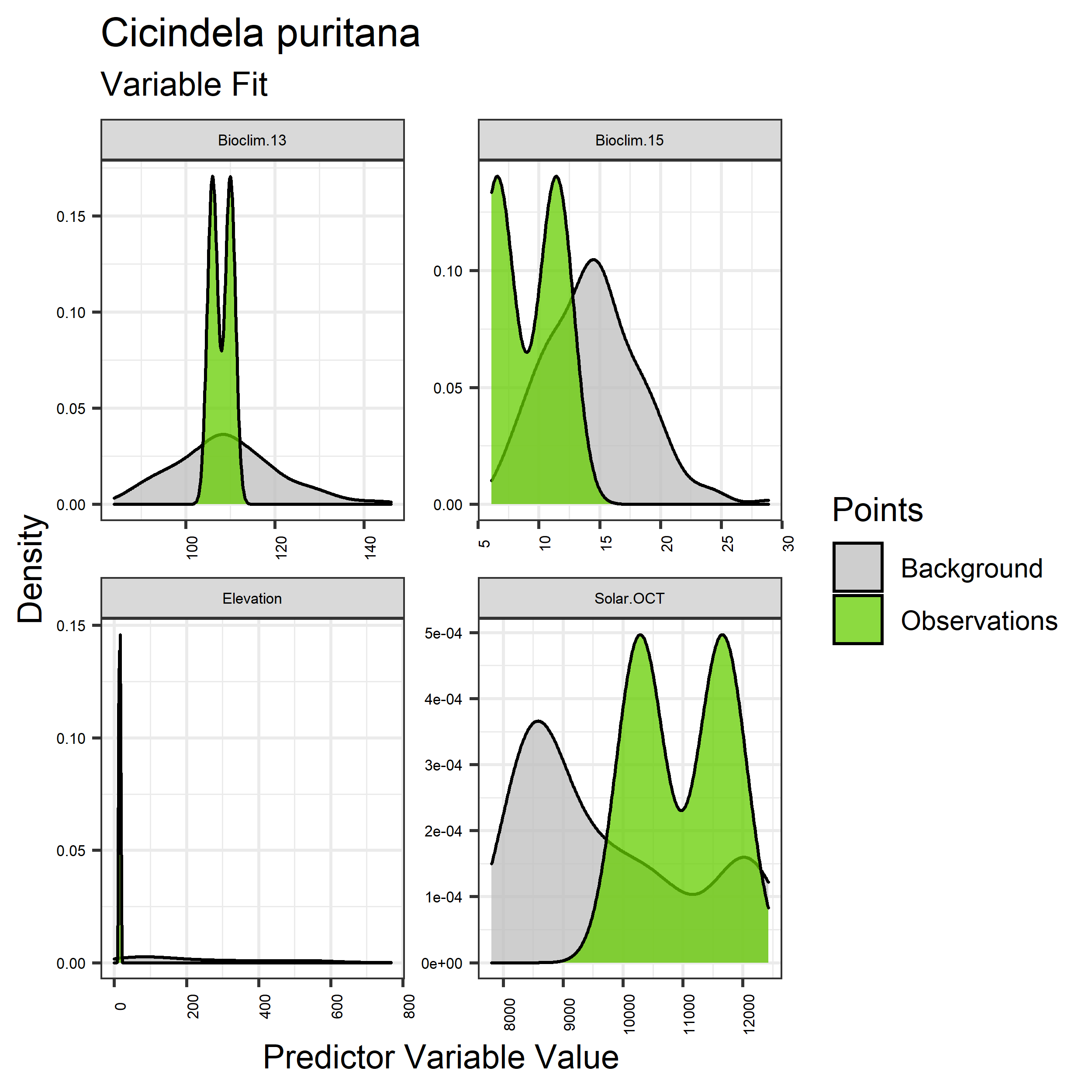
Figure 33. Sampling of continuous predictor variables retained in the best-fit Cicindela puritana distribution models. Distribution of each variable at points of species occurrence (green) are contrasted with points sampled across the full modeled extent (gray).
|
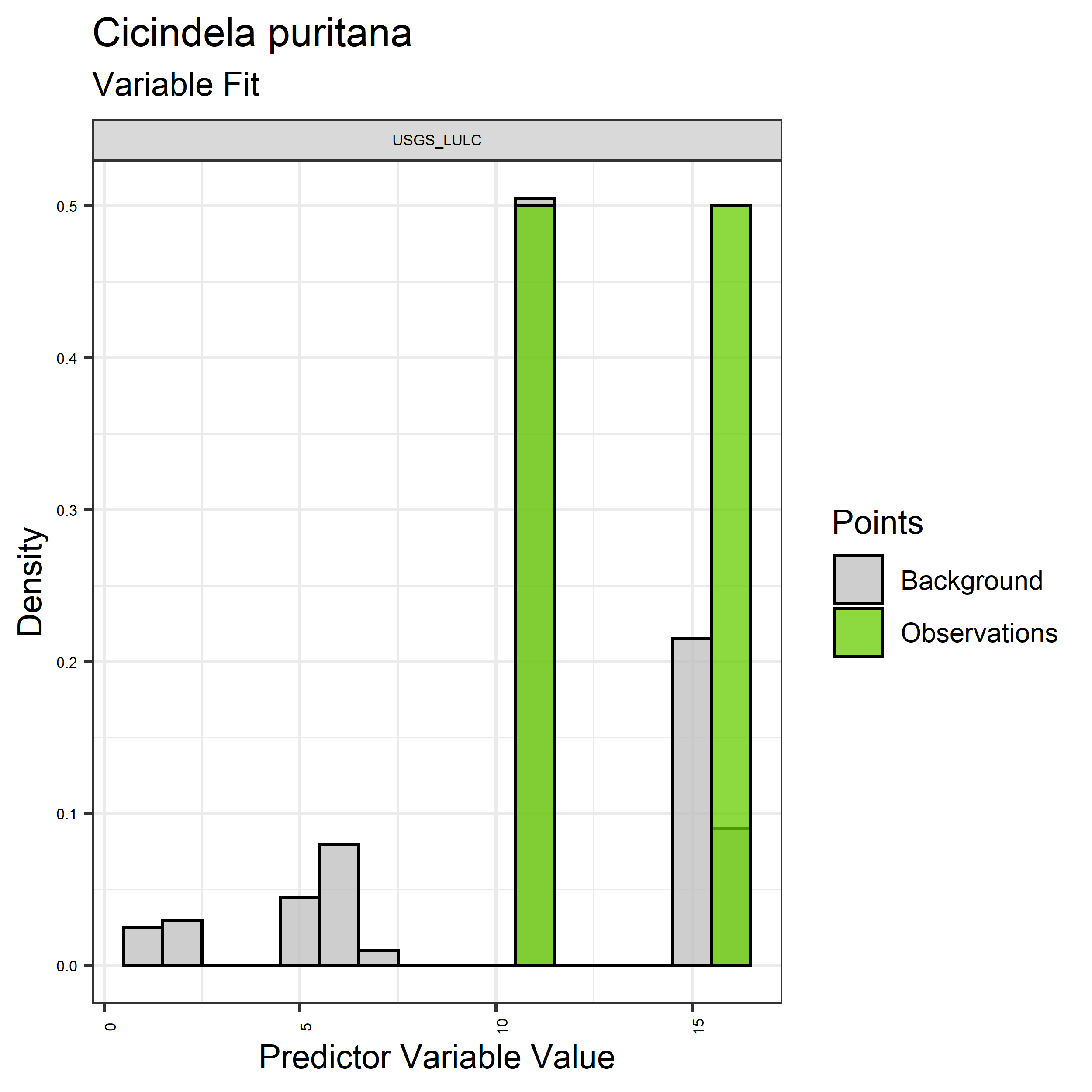
Figure 34. Sampling of discrete predictor variables retained in the best-fit Cicindela puritana distribution models. Distribution of each variable at points of species occurrence (green) are contrasted with points sampled across the full modeled extent.
|
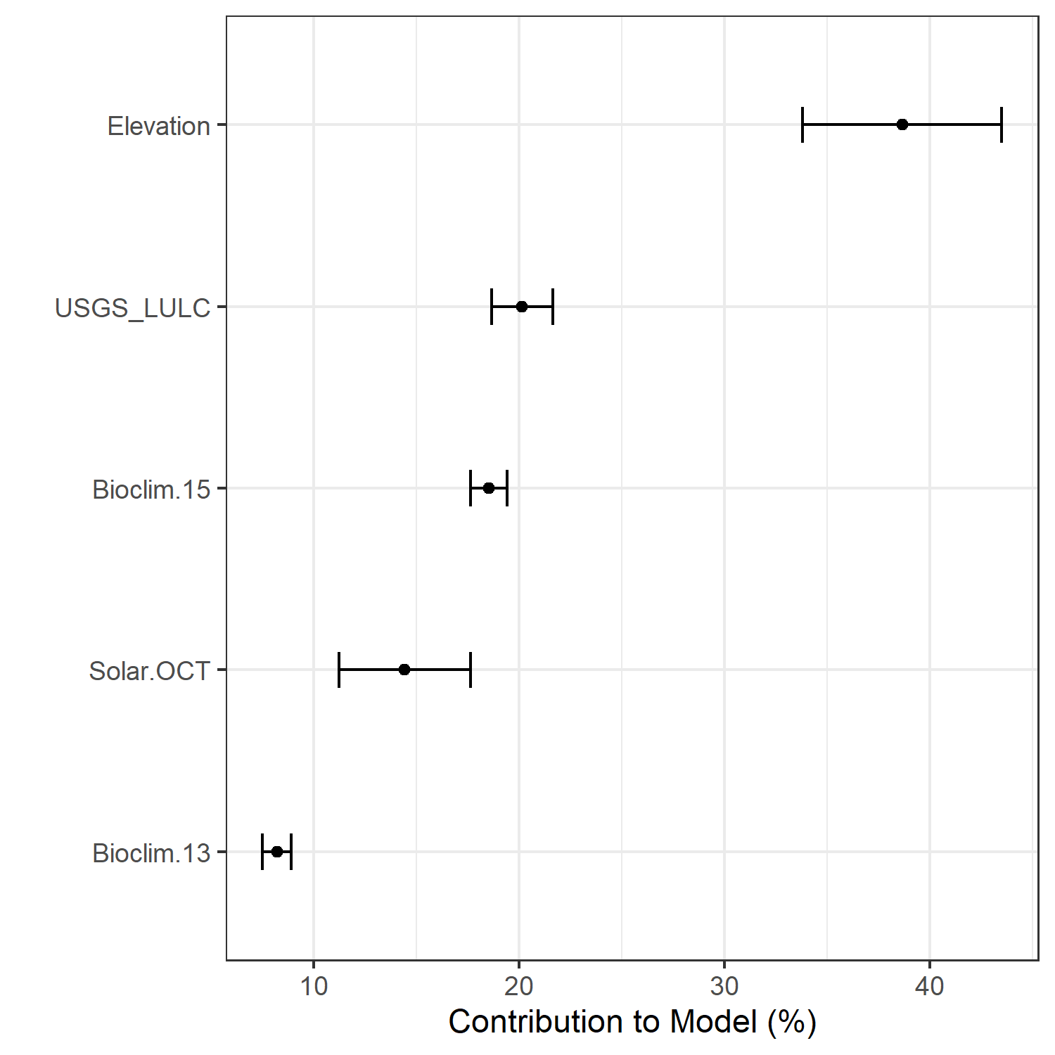
Figure 35. Percent contribution of each variable to best-fit species distribution models for Cicindela puritana. Values sum to 1.0.
|
Table 18. Mean Area Under Curve (AUC) for five realizations of the best-fit SDM for Cicindela puritana, calculated using 20% of species location records reserved for final evaluation.
| V1 |
V2 |
V3 |
V4 |
V5 |
mean |
sd |
| 0.9925 |
0.9925 |
0.9925 |
0.995 |
0.9925 |
0.993 |
0.00119 |
|
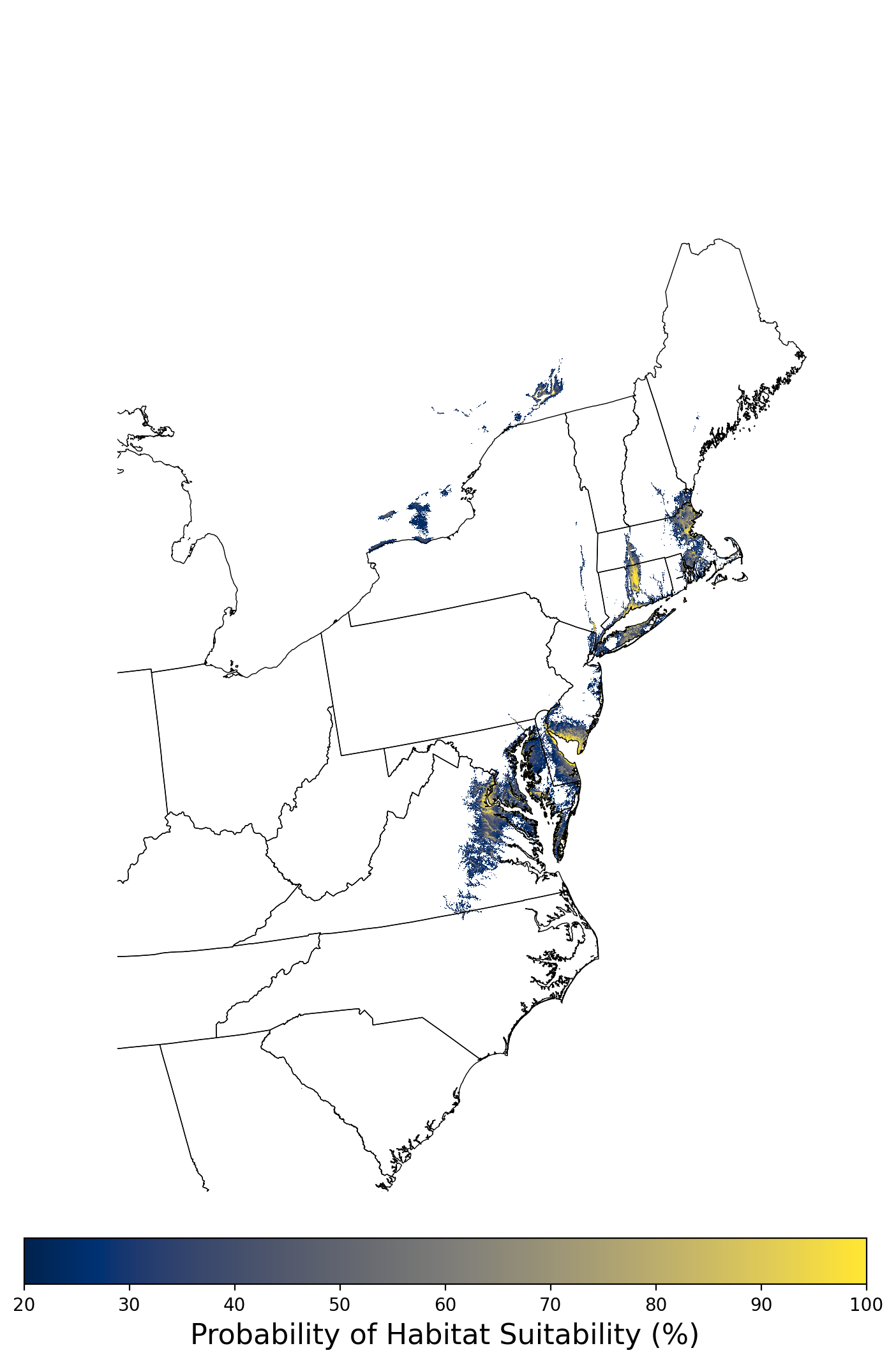
Figure 36. Final mean SDM output for Cicindela puritana. |
2.2.6 Species Distribution Modeling Results for Eurycea tonkawae
The species distribution modeling results consist of the following figures and tables:
- A table showing the SDM inputs (Table 19)
- A map showing the extent of SDM coverage (Figure 37)
- A graph showing the correlation between the predictor variable selected for evaluation (Figure 38)
- A graph of the model fit of each SDM iteration as measured by total Area Under Curve (AUC) where the curve is the Receiver Operating Curve, based on training data (Figure 39)
- A table showing the diagnostic statistics of the training data used in the final selected SDM iteration (Table 20)
- Graphs illustrating the predictor variable values sampled by the species observations and randomly selected background locations for continuous variables (Figure 40), and discrete variables (Figure 41)
- A graph showing the percent contribution of each predictor variable to the final selected SDM (Figure 42)
- A table showing the mean AUC for each of the five model runs that are averaged for the final selected SDM (Table 21)
- A map of the final averaged SDM (Figure 43)
Table 19. Input parameters for species distribution modeling of Eurycea tonkawae.
| Number of predictors |
33 |
| Names of predictors |
Bioclim.01.tif, Bioclim.02.tif, Bioclim.03.tif, Bioclim.04.tif,
Bioclim.05.tif, Bioclim.06.tif, Bioclim.07.tif, Bioclim.08.tif,
Bioclim.09.tif, Bioclim.10.tif, Bioclim.11.tif, Bioclim.12.tif,
Bioclim.13.tif, Bioclim.14.tif, Bioclim.15.tif, Bioclim.16.tif,
Bioclim.17.tif, Bioclim.18.tif, Bioclim.19.tif, Elevation.tif,
Solar.APR.tif, Solar.AUG.tif, Solar.DEC.tif, Solar.FEB.tif,
Solar.JAN.tif, Solar.JUL.tif, Solar.JUN.tif, Solar.MAR.tif,
Solar.MAY.tif, Solar.NOV.tif, Solar.OCT.tif, Solar.SEP.tif,
USGS_LULC.tif |
| Predictor correlation threshold |
0.67 |
| Predictor contribution threshold |
1.0 |
| SDM threshold |
0.2 |
| Number of iterations conducted |
5 |
| Final SDM iteration number |
4 |
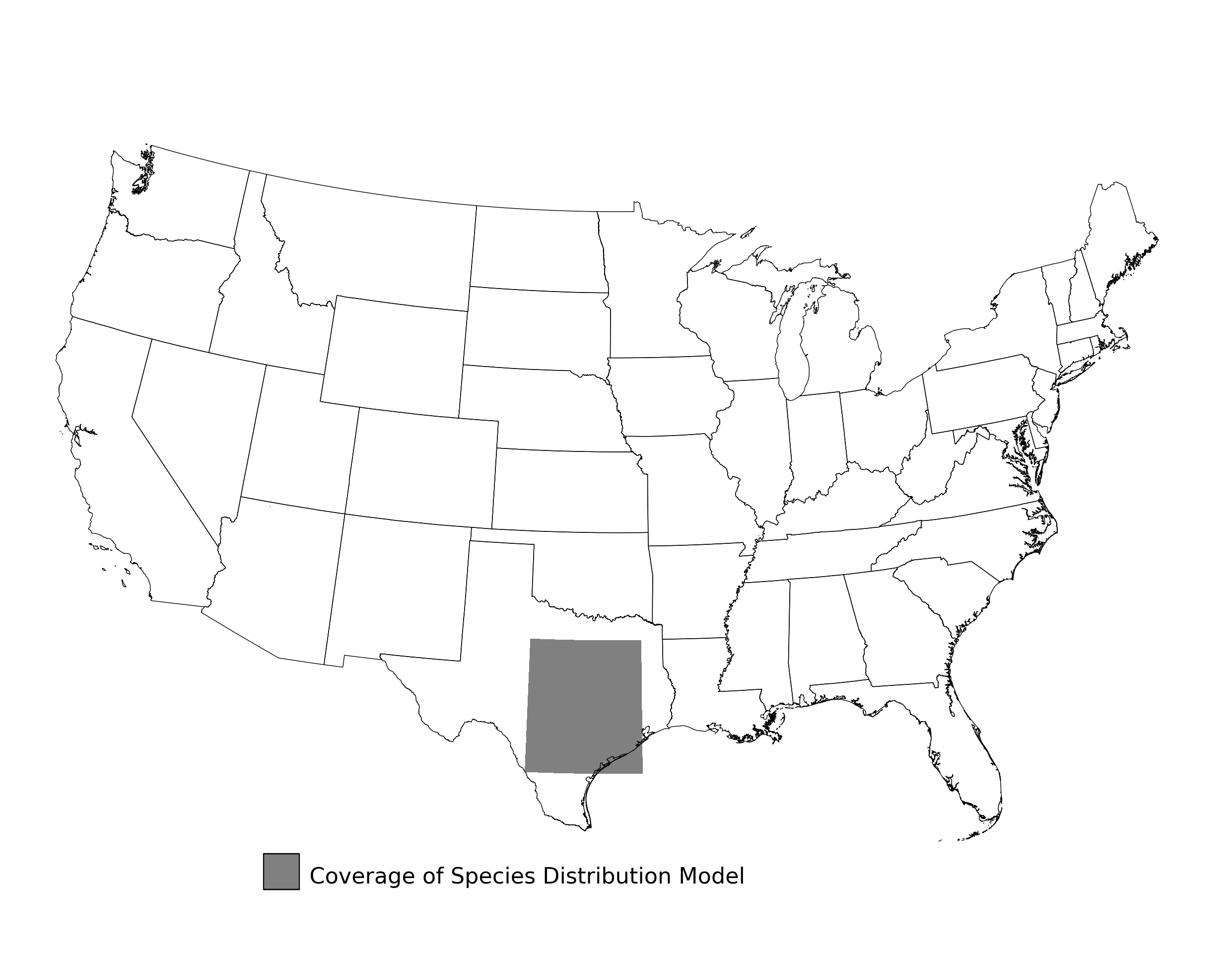
Figure 37. Extent of the species range modeled for Eurycea tonkawae. Modeling extent is determined by buffering species location records in all directions by 3 degrees latitude/longitude.
|
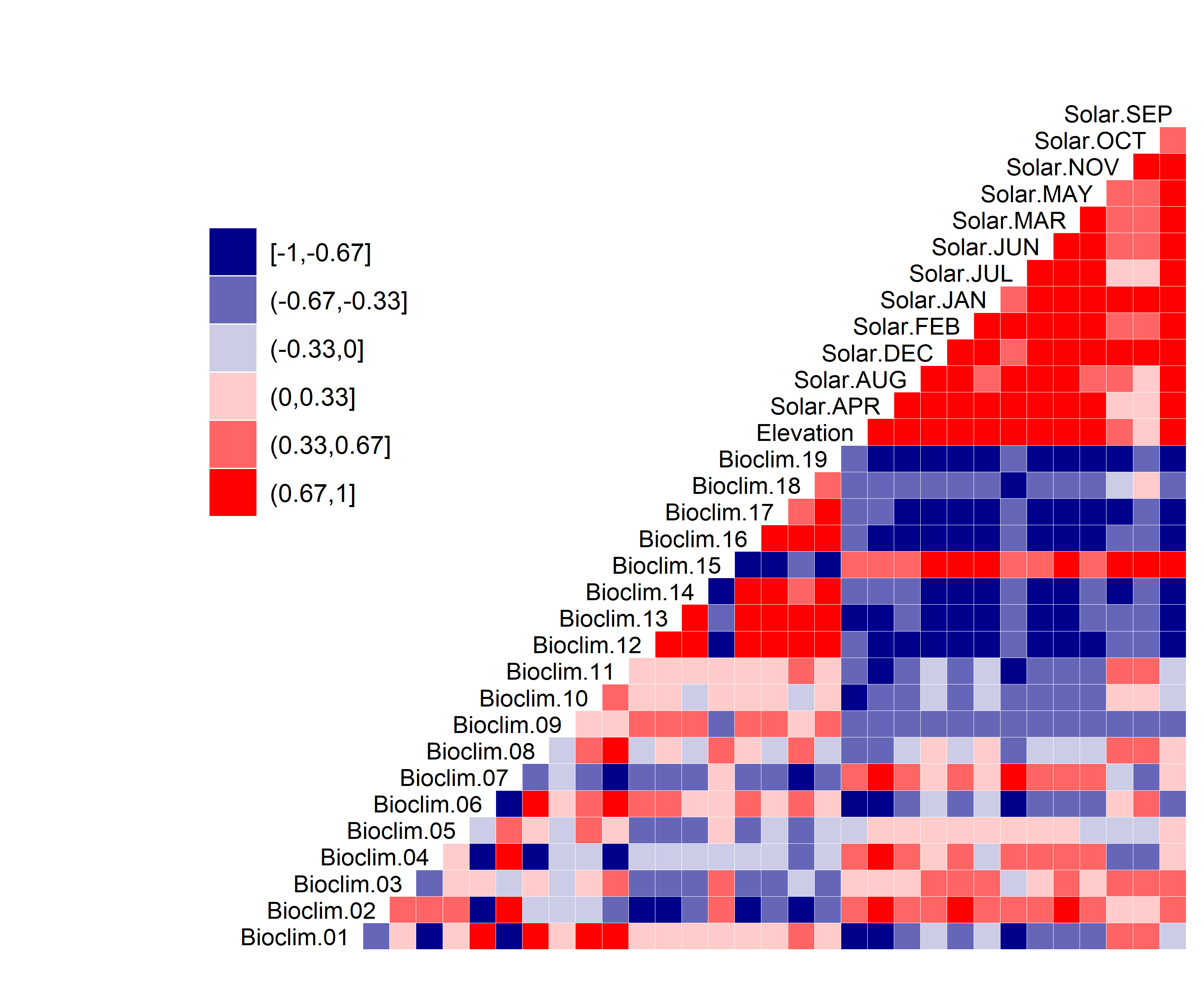
Figure 38. Correlation between SDM predictor variables for Eurycea tonkawae.
|
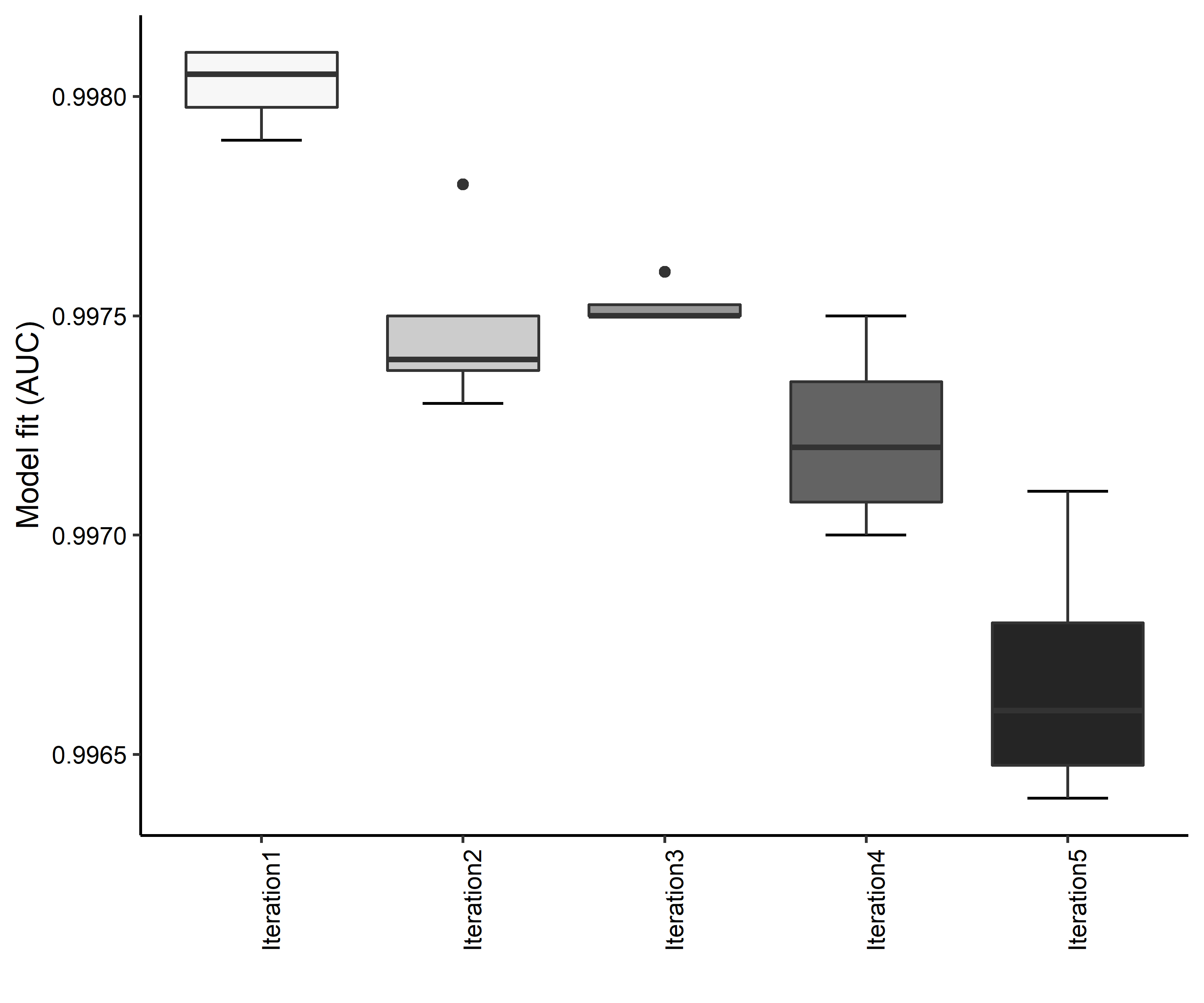
Figure 39. Boxplots of model fit for each iteration of Eurycea tonkawae distribution modeling. Statistics are calculated using 80% of species location records reserved for model training.
|
Table 20. Diagnostic statistics of the training data used in SDM iteration #4 for Eurycea tonkawae.
| Model Output |
Realization 1 |
Realization 2 |
Realization 3 |
Realization 4 |
Realization 5 |
Mean |
Standard Deviation |
| Number of training samples |
33.0000 |
33.0000 |
33.0000 |
33.0000 |
33.0000 |
33.00000 |
0.000000 |
| Regularized training gain |
4.2303 |
4.2856 |
4.3286 |
4.4054 |
4.2672 |
4.30342 |
0.067101 |
| Unregularized training gain |
4.7600 |
4.8274 |
4.8880 |
4.9784 |
4.7857 |
4.84790 |
0.087541 |
| Iterations |
500.0000 |
500.0000 |
500.0000 |
500.0000 |
500.0000 |
500.00000 |
0.000000 |
| Training AUC |
0.9969 |
0.9971 |
0.9973 |
0.9975 |
0.9970 |
0.99716 |
0.000241 |
| Number of background points |
10033.0000 |
10033.0000 |
10033.0000 |
10033.0000 |
10033.0000 |
10033.00000 |
0.000000 |
| Bioclim 02 contribution |
25.5542 |
34.0266 |
33.3664 |
32.8510 |
31.3142 |
31.42248 |
3.429627 |
| Bioclim 03 contribution |
23.0713 |
18.3111 |
19.4127 |
19.9869 |
19.7121 |
20.09882 |
1.779355 |
| Bioclim 04 contribution |
14.7605 |
11.0262 |
10.2769 |
10.8951 |
12.0286 |
11.79746 |
1.771597 |
| Elevation contribution |
29.4883 |
29.3298 |
29.1463 |
29.5880 |
28.6350 |
29.23748 |
0.376030 |
| USGS_LULC contribution |
7.1256 |
7.3064 |
7.7977 |
6.6789 |
8.3101 |
7.44374 |
0.628674 |
| Bioclim 02 permutation importance |
20.8513 |
22.9147 |
21.3880 |
26.4902 |
51.1133 |
28.55150 |
12.802989 |
| Bioclim 03 permutation importance |
13.2808 |
13.8272 |
13.7653 |
7.2902 |
4.9245 |
10.61760 |
4.206696 |
| Bioclim 04 permutation importance |
4.1629 |
7.2656 |
3.0164 |
5.3111 |
5.4483 |
5.04086 |
1.585698 |
| Elevation permutation importance |
61.2411 |
55.4658 |
61.2590 |
60.4737 |
38.0706 |
55.30204 |
9.930423 |
| USGS_LULC permutation importance |
0.4640 |
0.5266 |
0.5713 |
0.4348 |
0.4433 |
0.48800 |
0.058807 |
| Entropy |
4.9854 |
4.9305 |
4.8871 |
4.8069 |
4.9549 |
4.91296 |
0.069339 |
| Prevalence average probability of presence over background sites |
0.0077 |
0.0073 |
0.0069 |
0.0064 |
0.0074 |
0.00714 |
0.000503 |
| Fixed cumulative value 1 cumulative threshold |
1.0000 |
1.0000 |
1.0000 |
1.0000 |
1.0000 |
1.00000 |
0.000000 |
| Fixed cumulative value 1 Cloglog threshold |
0.0019 |
0.0024 |
0.0018 |
0.0021 |
0.0018 |
0.00200 |
0.000255 |
| Fixed cumulative value 1 area |
0.1047 |
0.0894 |
0.1119 |
0.0915 |
0.1100 |
0.10150 |
0.010453 |
| Fixed cumulative value 1 training omission |
0.0000 |
0.0000 |
0.0000 |
0.0000 |
0.0000 |
0.00000 |
0.000000 |
| Fixed cumulative value 5 cumulative threshold |
5.0000 |
5.0000 |
5.0000 |
5.0000 |
5.0000 |
5.00000 |
0.000000 |
| Fixed cumulative value 5 Cloglog threshold |
0.0298 |
0.0294 |
0.0235 |
0.0251 |
0.0249 |
0.02654 |
0.002864 |
| Fixed cumulative value 5 area |
0.0295 |
0.0281 |
0.0314 |
0.0272 |
0.0301 |
0.02926 |
0.001653 |
| Fixed cumulative value 5 training omission |
0.0000 |
0.0000 |
0.0000 |
0.0000 |
0.0000 |
0.00000 |
0.000000 |
| Fixed cumulative value 10 cumulative threshold |
10.0000 |
10.0000 |
10.0000 |
10.0000 |
10.0000 |
10.00000 |
0.000000 |
| Fixed cumulative value 10 Cloglog threshold |
0.0841 |
0.0832 |
0.0714 |
0.0773 |
0.0817 |
0.07954 |
0.005247 |
| Fixed cumulative value 10 area |
0.0154 |
0.0151 |
0.0159 |
0.0144 |
0.0154 |
0.01524 |
0.000550 |
| Fixed cumulative value 10 training omission |
0.0303 |
0.0303 |
0.0303 |
0.0303 |
0.0303 |
0.03030 |
0.000000 |
| Minimum training presence cumulative threshold |
7.1911 |
7.3582 |
8.4887 |
8.3856 |
7.5680 |
7.79832 |
0.599373 |
| Minimum training presence Cloglog threshold |
0.0500 |
0.0554 |
0.0532 |
0.0606 |
0.0514 |
0.05412 |
0.004149 |
| Minimum training presence area |
0.0214 |
0.0202 |
0.0190 |
0.0171 |
0.0205 |
0.01964 |
0.001659 |
| Minimum training presence training omission |
0.0000 |
0.0000 |
0.0000 |
0.0000 |
0.0000 |
0.00000 |
0.000000 |
| X10 percentile training presence cumulative threshold |
22.2826 |
21.9492 |
26.1023 |
24.0051 |
24.0215 |
23.67214 |
1.661169 |
| X10 percentile training presence Cloglog threshold |
0.4060 |
0.3629 |
0.4570 |
0.3305 |
0.4497 |
0.40122 |
0.054668 |
| X10 percentile training presence area |
0.0064 |
0.0062 |
0.0048 |
0.0047 |
0.0055 |
0.00552 |
0.000779 |
| X10 percentile training presence training omission |
0.0909 |
0.0909 |
0.0909 |
0.0909 |
0.0909 |
0.09090 |
0.000000 |
| Equal training sensitivity and specificity cumulative threshold |
7.2267 |
7.4000 |
8.4887 |
8.4367 |
7.6054 |
7.83150 |
0.591877 |
| Equal training sensitivity and specificity Cloglog threshold |
0.0506 |
0.0562 |
0.0532 |
0.0607 |
0.0517 |
0.05448 |
0.004064 |
| Equal training sensitivity and specificity area |
0.0214 |
0.0202 |
0.0190 |
0.0170 |
0.0205 |
0.01962 |
0.001698 |
| Equal training sensitivity and specificity training omission |
0.0303 |
0.0303 |
0.0303 |
0.0303 |
0.0303 |
0.03030 |
0.000000 |
| Maximum training sensitivity plus specificity cumulative threshold |
7.1911 |
7.3582 |
8.4887 |
8.3856 |
7.5680 |
7.79832 |
0.599373 |
| Maximum training sensitivity plus specificity Cloglog threshold |
0.0500 |
0.0554 |
0.0532 |
0.0606 |
0.0514 |
0.05412 |
0.004149 |
| Maximum training sensitivity plus specificity area |
0.0214 |
0.0202 |
0.0190 |
0.0171 |
0.0205 |
0.01964 |
0.001659 |
| Maximum training sensitivity plus specificity training omission |
0.0000 |
0.0000 |
0.0000 |
0.0000 |
0.0000 |
0.00000 |
0.000000 |
| Balance training omission predicted area and threshold value cumulative threshold |
1.9561 |
1.7456 |
2.0349 |
1.7520 |
2.0096 |
1.89964 |
0.140624 |
| Balance training omission predicted area and threshold value Cloglog threshold |
0.0058 |
0.0055 |
0.0052 |
0.0049 |
0.0056 |
0.00540 |
0.000354 |
| Balance training omission predicted area and threshold value area |
0.0643 |
0.0615 |
0.0669 |
0.0630 |
0.0643 |
0.06400 |
0.001990 |
| Balance training omission predicted area and threshold value training omission |
0.0000 |
0.0000 |
0.0000 |
0.0000 |
0.0000 |
0.00000 |
0.000000 |
| Equate entropy of thresholded and original distributions cumulative threshold |
10.5663 |
10.9172 |
11.9114 |
11.6849 |
10.9418 |
11.20432 |
0.567746 |
| Equate entropy of thresholded and original distributions Cloglog threshold |
0.0884 |
0.0957 |
0.0966 |
0.0982 |
0.0988 |
0.09554 |
0.004178 |
| Equate entropy of thresholded and original distributions area |
0.0146 |
0.0138 |
0.0132 |
0.0122 |
0.0141 |
0.01358 |
0.000923 |
| Equate entropy of thresholded and original distributions training omission |
0.0303 |
0.0303 |
0.0303 |
0.0303 |
0.0303 |
0.03030 |
0.000000 |
|
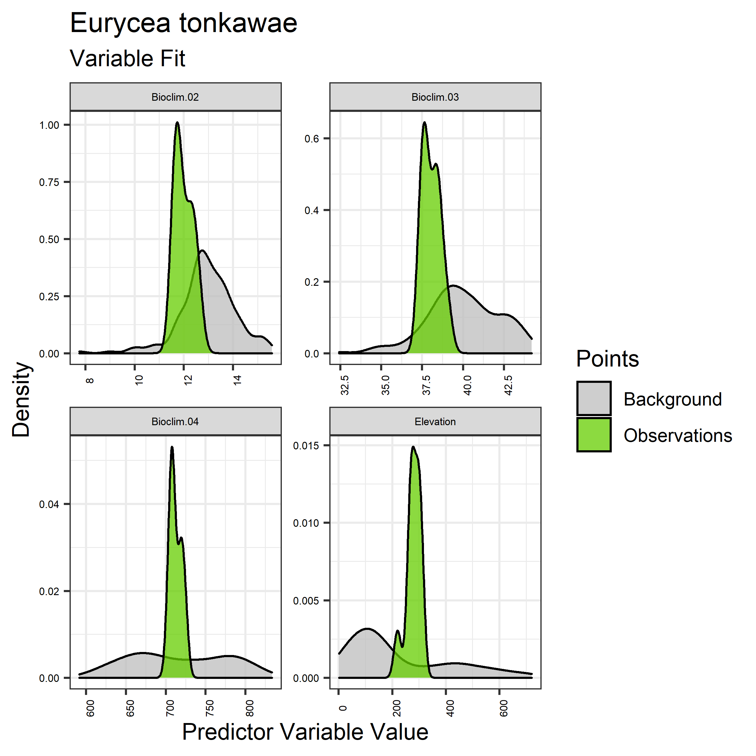
Figure 40. Sampling of continuous predictor variables retained in the best-fit Eurycea tonkawae distribution models. Distribution of each variable at points of species occurrence (green) are contrasted with points sampled across the full modeled extent (gray).
|
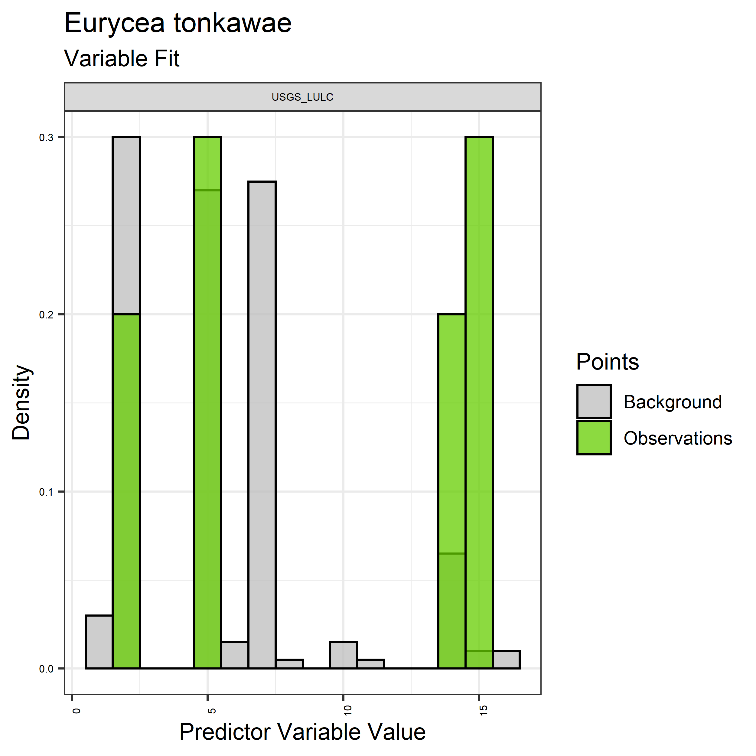
Figure 41. Sampling of discrete predictor variables retained in the best-fit Eurycea tonkawae distribution models. Distribution of each variable at points of species occurrence (green) are contrasted with points sampled across the full modeled extent.
|
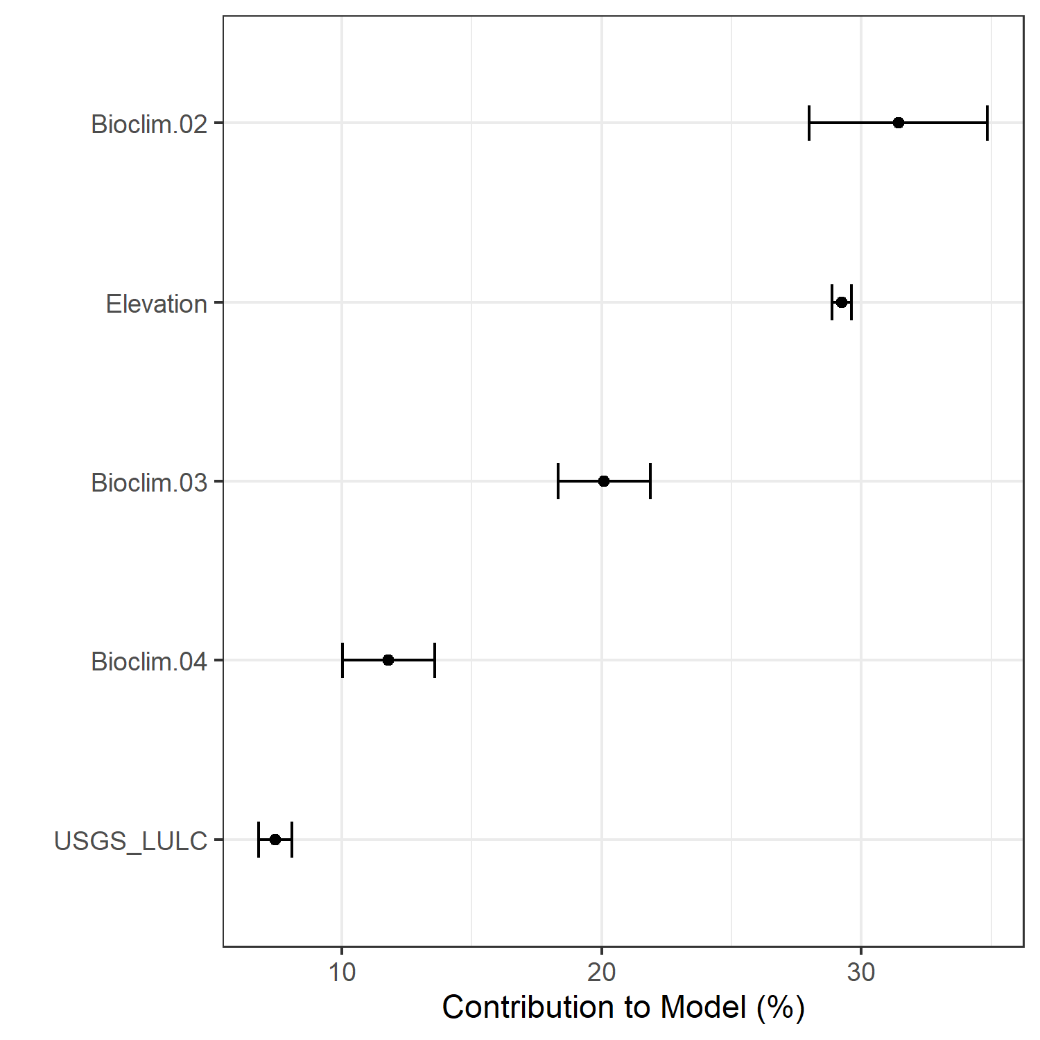
Figure 42. Percent contribution of each variable to best-fit species distribution models for Eurycea tonkawae. Values sum to 1.0.
|
Table 21. Mean Area Under Curve (AUC) for five realizations of the best-fit SDM for Eurycea tonkawae, calculated using 20% of species location records reserved for final evaluation.
| V1 |
V2 |
V3 |
V4 |
V5 |
mean |
sd |
| 0.9995 |
1 |
0.999 |
1 |
0.9995 |
0.9996 |
0.000411 |
|
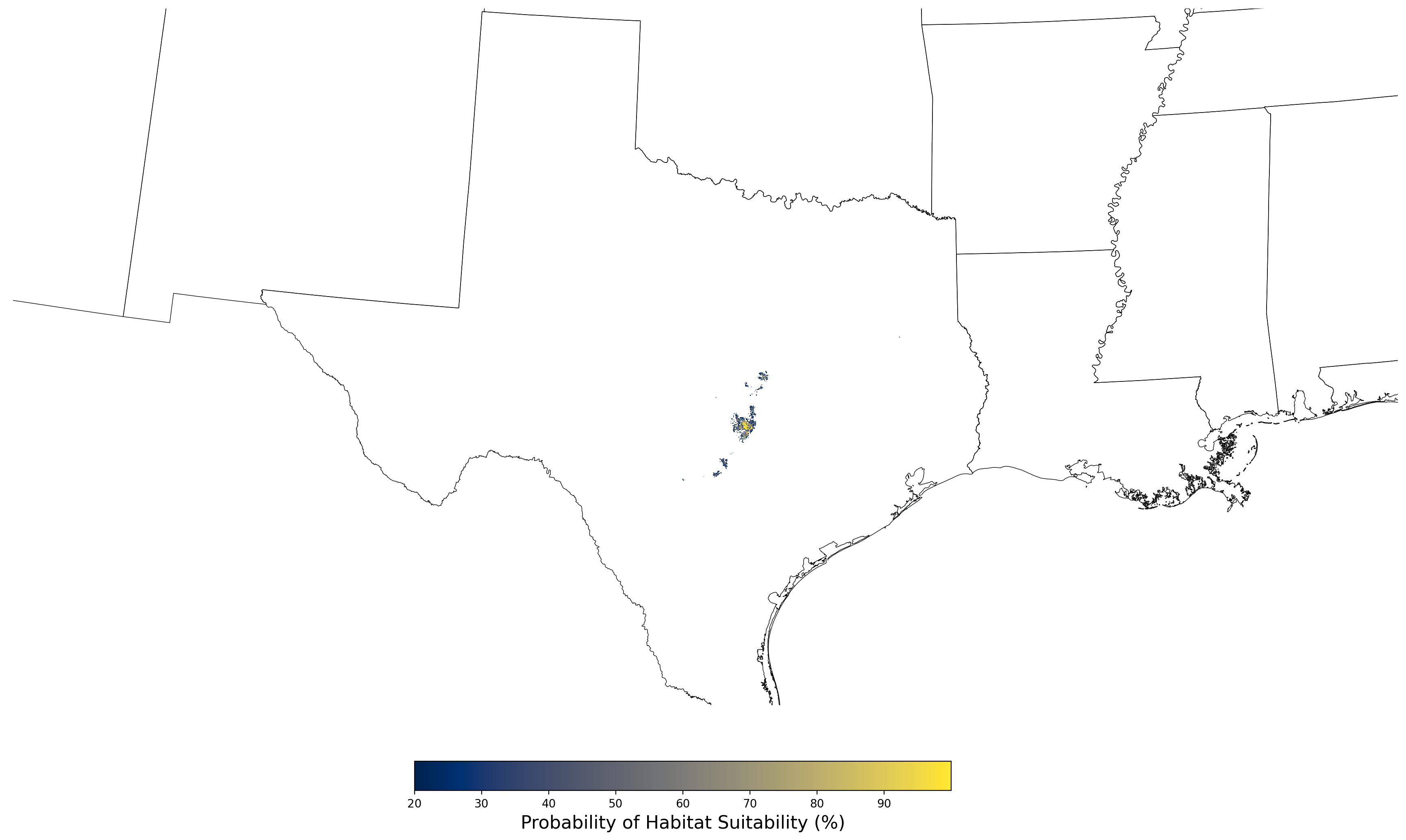
Figure 43. Final mean SDM output for Eurycea tonkawae. |
2.2.7 Species Distribution Modeling Results for Lycaeides melissa samuelis
The species distribution modeling results consist of the following figures and tables:
- A table showing the SDM inputs (Table 22)
- A map showing the extent of SDM coverage (Figure 44)
- A graph showing the correlation between the predictor variable selected for evaluation (Figure 45)
- A graph of the model fit of each SDM iteration as measured by total Area Under Curve (AUC) where the curve is the Receiver Operating Curve, based on training data (Figure 46)
- A table showing the diagnostic statistics of the training data used in the final selected SDM iteration (Table 23)
- Graphs illustrating the predictor variable values sampled by the species observations and randomly selected background locations for continuous variables (Figure 47), and discrete variables (Figure 48)
- A graph showing the percent contribution of each predictor variable to the final selected SDM (Figure 49)
- A table showing the mean AUC for each of the five model runs that are averaged for the final selected SDM (Table 24)
- A map of the final averaged SDM (Figure 50)
Table 22. Input parameters for species distribution modeling of Lycaeides melissa samuelis.
| Number of predictors |
32 |
| Names of predictors |
Bioclim.01.tif, Bioclim.02.tif, Bioclim.03.tif, Bioclim.04.tif,
Bioclim.05.tif, Bioclim.06.tif, Bioclim.07.tif, Bioclim.08.tif,
Bioclim.09.tif, Bioclim.10.tif, Bioclim.11.tif, Bioclim.12.tif,
Bioclim.13.tif, Bioclim.14.tif, Bioclim.15.tif, Bioclim.16.tif,
Bioclim.17.tif, Bioclim.18.tif, Bioclim.19.tif, Elevation.tif,
Solar.APR.tif, Solar.AUG.tif, Solar.DEC.tif, Solar.FEB.tif,
Solar.JAN.tif, Solar.JUL.tif, Solar.JUN.tif, Solar.MAR.tif,
Solar.MAY.tif, Solar.NOV.tif, Solar.OCT.tif, Solar.SEP.tif |
| Predictor correlation threshold |
0.67 |
| Predictor contribution threshold |
1.0 |
| SDM threshold |
0.2 |
| Number of iterations conducted |
3 |
| Final SDM iteration number |
2 |
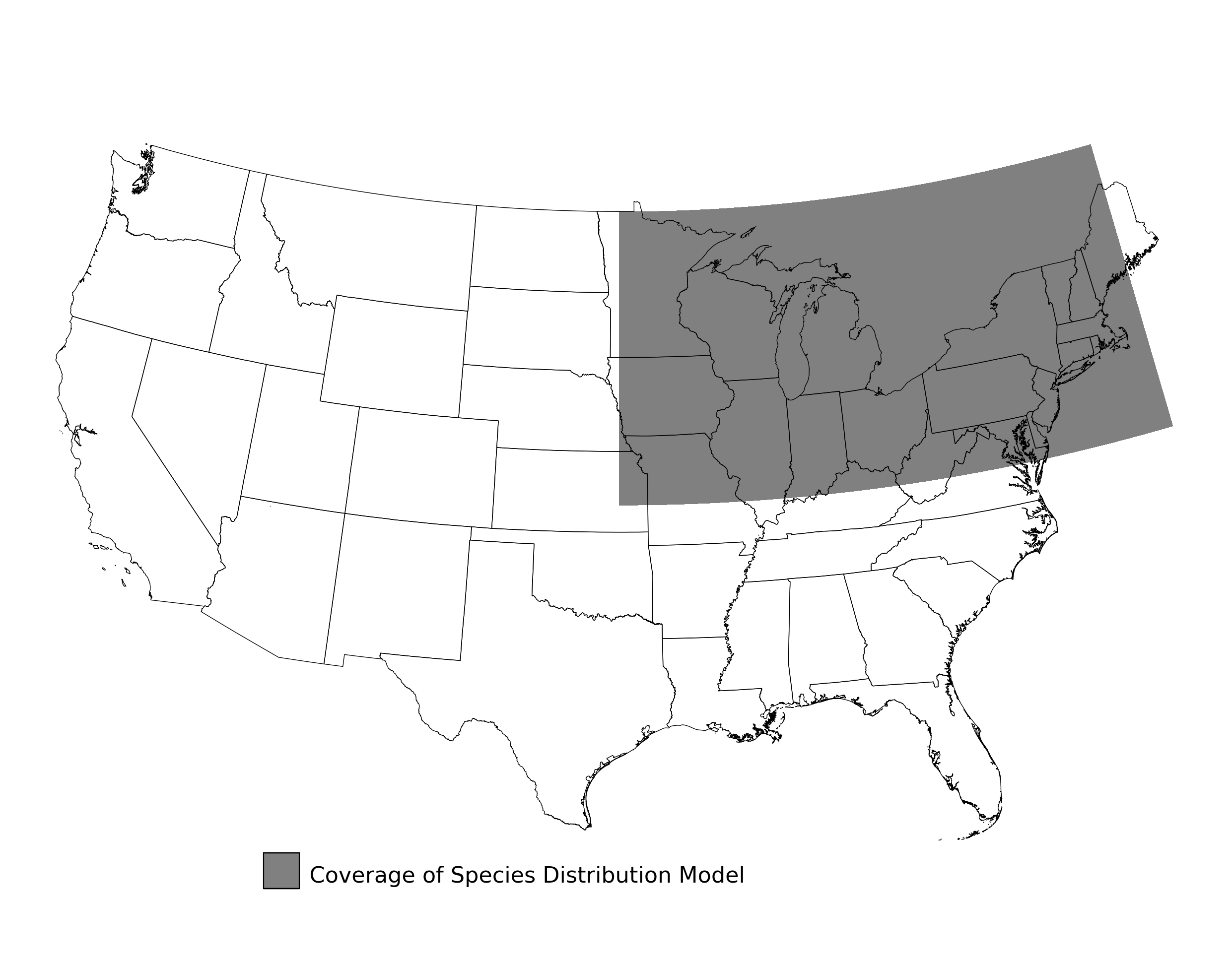
Figure 44. Extent of the species range modeled for Lycaeides melissa samuelis. Modeling extent is determined by buffering species location records in all directions by 3 degrees latitude/longitude.
|
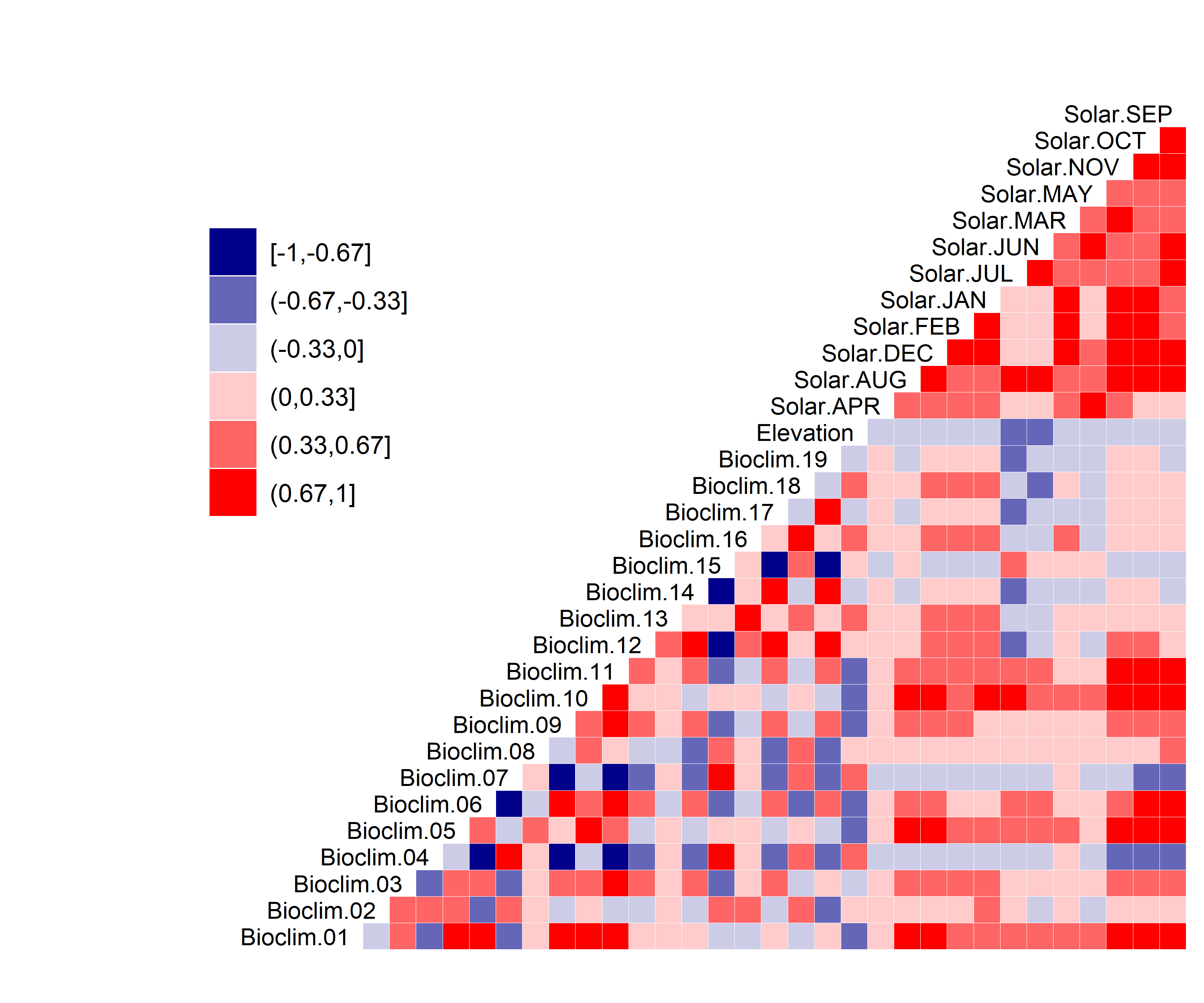
Figure 45. Correlation between SDM predictor variables for Lycaeides melissa samuelis.
|
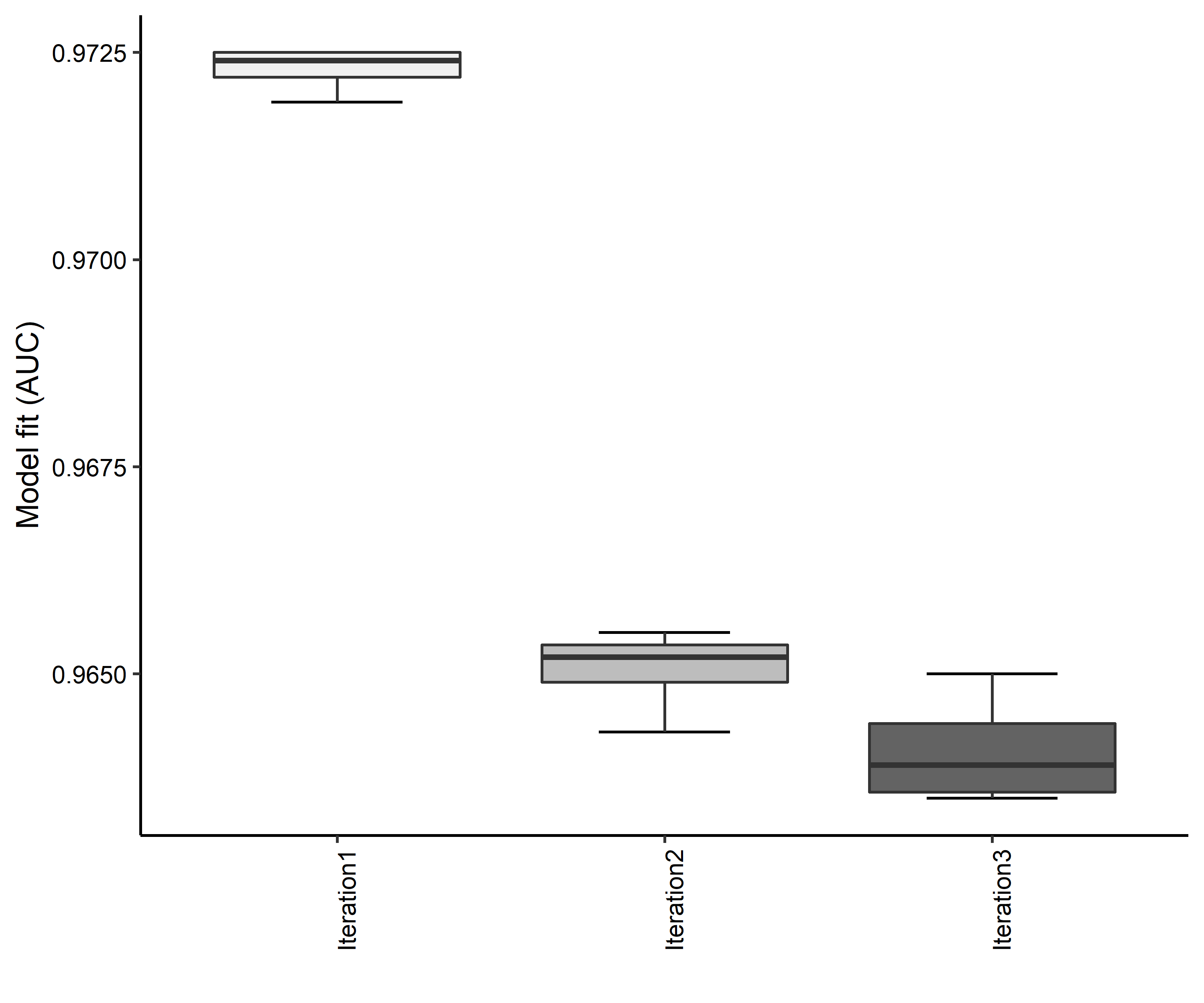
Figure 46. Boxplots of model fit for each iteration of Lycaeides melissa samuelis distribution modeling. Statistics are calculated using 80% of species location records reserved for model training.
|
Table 23. Diagnostic statistics of the training data used in SDM iteration #2 for Lycaeides melissa samuelis.
| Model Output |
Realization 1 |
Realization 2 |
Realization 3 |
Realization 4 |
Realization 5 |
Mean |
Standard Deviation |
| Number of training samples |
437.0000 |
437.0000 |
437.0000 |
437.0000 |
437.0000 |
437.00000 |
0.000000 |
| Regularized training gain |
2.1456 |
2.1028 |
2.1428 |
2.0984 |
2.1371 |
2.12534 |
0.022844 |
| Unregularized training gain |
2.2867 |
2.2427 |
2.2935 |
2.2512 |
2.2874 |
2.27230 |
0.023485 |
| Iterations |
500.0000 |
500.0000 |
500.0000 |
500.0000 |
500.0000 |
500.00000 |
0.000000 |
| Training AUC |
0.9614 |
0.9598 |
0.9612 |
0.9600 |
0.9617 |
0.96082 |
0.000861 |
| Number of background points |
10437.0000 |
10437.0000 |
10437.0000 |
10437.0000 |
10437.0000 |
10437.00000 |
0.000000 |
| Bioclim 03 contribution |
12.6731 |
11.7635 |
12.2901 |
12.4987 |
12.0450 |
12.25408 |
0.360935 |
| Bioclim 08 contribution |
3.9398 |
3.9605 |
4.8659 |
4.3553 |
4.6065 |
4.34560 |
0.403686 |
| Bioclim 13 contribution |
7.9622 |
8.2222 |
7.6018 |
8.5993 |
7.1175 |
7.90060 |
0.569634 |
| Bioclim 15 contribution |
17.2558 |
17.2404 |
16.7304 |
17.7439 |
17.5796 |
17.31002 |
0.388803 |
| Solar MAR contribution |
6.3224 |
6.4639 |
6.8737 |
6.6805 |
6.3526 |
6.53862 |
0.234172 |
| Solar OCT contribution |
51.8467 |
52.3495 |
51.6380 |
50.1223 |
52.2988 |
51.65106 |
0.905944 |
| Bioclim 03 permutation importance |
22.9672 |
19.4589 |
19.1587 |
22.7873 |
23.9274 |
21.65990 |
2.192146 |
| Bioclim 08 permutation importance |
2.1299 |
1.7362 |
2.3897 |
2.3814 |
2.7276 |
2.27296 |
0.367649 |
| Bioclim 13 permutation importance |
12.9875 |
12.9077 |
11.1657 |
13.6872 |
12.5514 |
12.65990 |
0.931192 |
| Bioclim 15 permutation importance |
4.8413 |
4.0114 |
4.3679 |
5.1806 |
4.2302 |
4.52628 |
0.475716 |
| Solar MAR permutation importance |
13.8101 |
14.3228 |
14.7914 |
16.0334 |
15.9142 |
14.97438 |
0.977033 |
| Solar OCT permutation importance |
43.2640 |
47.5631 |
48.1265 |
39.9301 |
40.6493 |
43.90660 |
3.808315 |
| Entropy |
7.1093 |
7.1530 |
7.1121 |
7.1555 |
7.1187 |
7.12972 |
0.022669 |
| Prevalence average probability of presence over background sites |
0.0672 |
0.0702 |
0.0671 |
0.0704 |
0.0675 |
0.06848 |
0.001669 |
| Fixed cumulative value 1 cumulative threshold |
1.0000 |
1.0000 |
1.0000 |
1.0000 |
1.0000 |
1.00000 |
0.000000 |
| Fixed cumulative value 1 Cloglog threshold |
0.0146 |
0.0145 |
0.0144 |
0.0144 |
0.0140 |
0.01438 |
0.000228 |
| Fixed cumulative value 1 area |
0.2699 |
0.2850 |
0.2804 |
0.2778 |
0.2826 |
0.27914 |
0.005811 |
| Fixed cumulative value 1 training omission |
0.0069 |
0.0046 |
0.0046 |
0.0069 |
0.0069 |
0.00598 |
0.001260 |
| Fixed cumulative value 5 cumulative threshold |
5.0000 |
5.0000 |
5.0000 |
5.0000 |
5.0000 |
5.00000 |
0.000000 |
| Fixed cumulative value 5 Cloglog threshold |
0.0784 |
0.0786 |
0.0749 |
0.0854 |
0.0748 |
0.07842 |
0.004308 |
| Fixed cumulative value 5 area |
0.1446 |
0.1514 |
0.1517 |
0.1493 |
0.1519 |
0.14978 |
0.003077 |
| Fixed cumulative value 5 training omission |
0.0366 |
0.0343 |
0.0343 |
0.0343 |
0.0320 |
0.03430 |
0.001626 |
| Fixed cumulative value 10 cumulative threshold |
10.0000 |
10.0000 |
10.0000 |
10.0000 |
10.0000 |
10.00000 |
0.000000 |
| Fixed cumulative value 10 Cloglog threshold |
0.1738 |
0.1729 |
0.1563 |
0.1781 |
0.1627 |
0.16876 |
0.008969 |
| Fixed cumulative value 10 area |
0.0988 |
0.1030 |
0.1008 |
0.1044 |
0.1012 |
0.10164 |
0.002147 |
| Fixed cumulative value 10 training omission |
0.0641 |
0.0664 |
0.0641 |
0.0664 |
0.0686 |
0.06592 |
0.001889 |
| Minimum training presence cumulative threshold |
0.0465 |
0.0578 |
0.0550 |
0.0973 |
0.0818 |
0.06768 |
0.021117 |
| Minimum training presence Cloglog threshold |
0.0009 |
0.0011 |
0.0010 |
0.0017 |
0.0014 |
0.00122 |
0.000327 |
| Minimum training presence area |
0.4870 |
0.4949 |
0.4955 |
0.4558 |
0.4768 |
0.48200 |
0.016486 |
| Minimum training presence training omission |
0.0000 |
0.0000 |
0.0000 |
0.0000 |
0.0000 |
0.00000 |
0.000000 |
| X10 percentile training presence cumulative threshold |
18.8231 |
17.2822 |
17.8544 |
17.8848 |
17.8019 |
17.92928 |
0.557099 |
| X10 percentile training presence Cloglog threshold |
0.3815 |
0.3638 |
0.3644 |
0.3695 |
0.3686 |
0.36956 |
0.007129 |
| X10 percentile training presence area |
0.0653 |
0.0724 |
0.0673 |
0.0713 |
0.0689 |
0.06904 |
0.002891 |
| X10 percentile training presence training omission |
0.0984 |
0.0984 |
0.0984 |
0.0984 |
0.0984 |
0.09840 |
0.000000 |
| Equal training sensitivity and specificity cumulative threshold |
14.6561 |
14.4018 |
14.4709 |
15.1887 |
14.7213 |
14.68776 |
0.308978 |
| Equal training sensitivity and specificity Cloglog threshold |
0.2905 |
0.2816 |
0.2664 |
0.2933 |
0.2902 |
0.28440 |
0.010976 |
| Equal training sensitivity and specificity area |
0.0772 |
0.0816 |
0.0778 |
0.0797 |
0.0781 |
0.07888 |
0.001780 |
| Equal training sensitivity and specificity training omission |
0.0778 |
0.0824 |
0.0778 |
0.0801 |
0.0778 |
0.07918 |
0.002057 |
| Maximum training sensitivity plus specificity cumulative threshold |
15.3555 |
14.4018 |
15.8409 |
14.8946 |
14.7213 |
15.04282 |
0.563682 |
| Maximum training sensitivity plus specificity Cloglog threshold |
0.3076 |
0.2816 |
0.3056 |
0.2860 |
0.2902 |
0.29420 |
0.011742 |
| Maximum training sensitivity plus specificity area |
0.0748 |
0.0816 |
0.0730 |
0.0808 |
0.0781 |
0.07766 |
0.003724 |
| Maximum training sensitivity plus specificity training omission |
0.0778 |
0.0801 |
0.0801 |
0.0755 |
0.0778 |
0.07826 |
0.001924 |
| Balance training omission predicted area and threshold value cumulative threshold |
1.4862 |
1.3510 |
1.8675 |
1.6217 |
1.5032 |
1.56592 |
0.193998 |
| Balance training omission predicted area and threshold value Cloglog threshold |
0.0215 |
0.0192 |
0.0266 |
0.0236 |
0.0210 |
0.02238 |
0.002832 |
| Balance training omission predicted area and threshold value area |
0.2383 |
0.2594 |
0.2294 |
0.2374 |
0.2482 |
0.24254 |
0.011547 |
| Balance training omission predicted area and threshold value training omission |
0.0069 |
0.0046 |
0.0114 |
0.0069 |
0.0069 |
0.00734 |
0.002479 |
| Equate entropy of thresholded and original distributions cumulative threshold |
7.4836 |
7.5368 |
7.9199 |
7.4914 |
7.8712 |
7.66058 |
0.216144 |
| Equate entropy of thresholded and original distributions Cloglog threshold |
0.1257 |
0.1227 |
0.1188 |
0.1337 |
0.1195 |
0.12408 |
0.006040 |
| Equate entropy of thresholded and original distributions area |
0.1172 |
0.1224 |
0.1175 |
0.1227 |
0.1182 |
0.11960 |
0.002719 |
| Equate entropy of thresholded and original distributions training omission |
0.0481 |
0.0503 |
0.0458 |
0.0503 |
0.0412 |
0.04714 |
0.003807 |
|
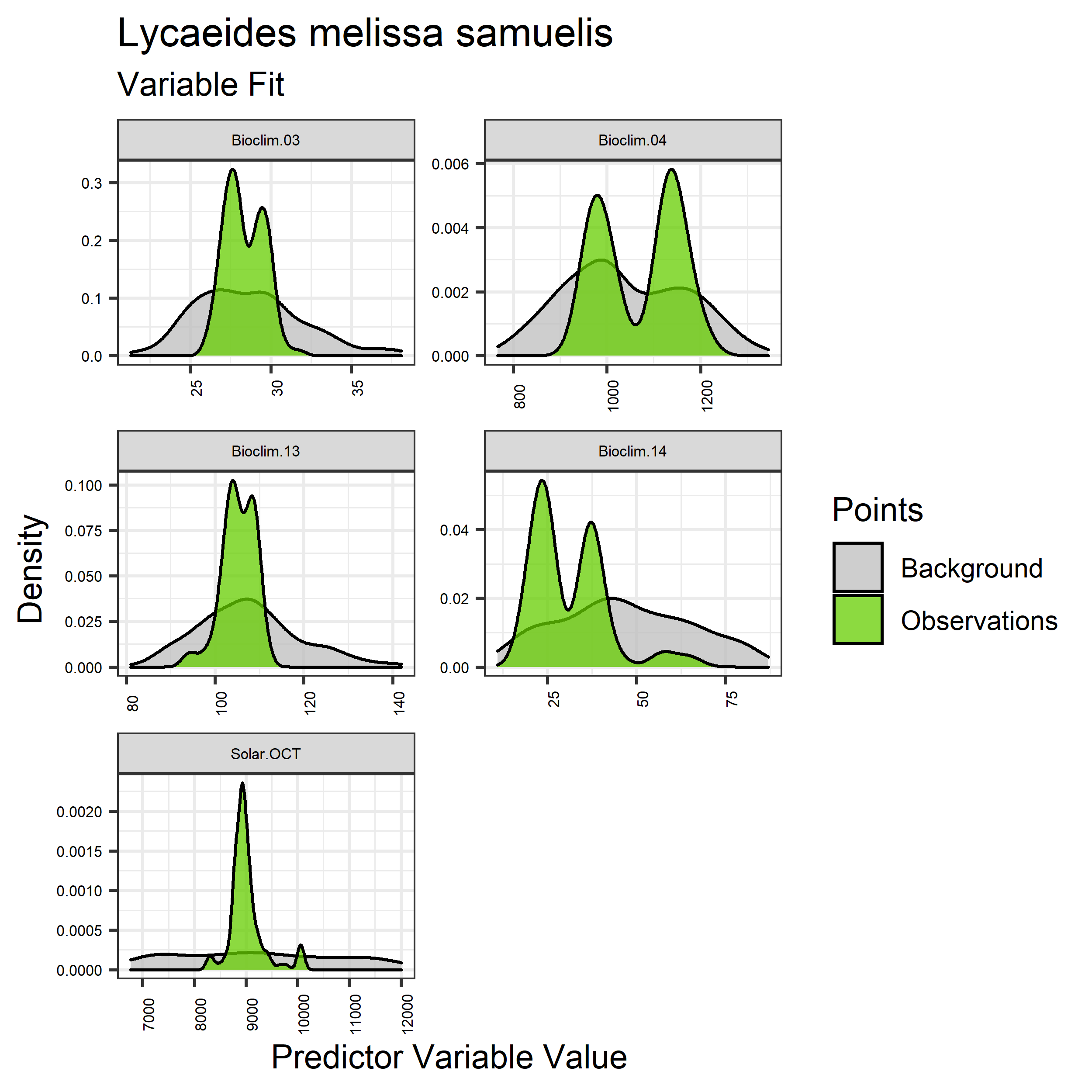
Figure 47. Sampling of continuous predictor variables retained in the best-fit Lycaeides melissa samuelis distribution models. Distribution of each variable at points of species occurrence (green) are contrasted with points sampled across the full modeled extent (gray).
|
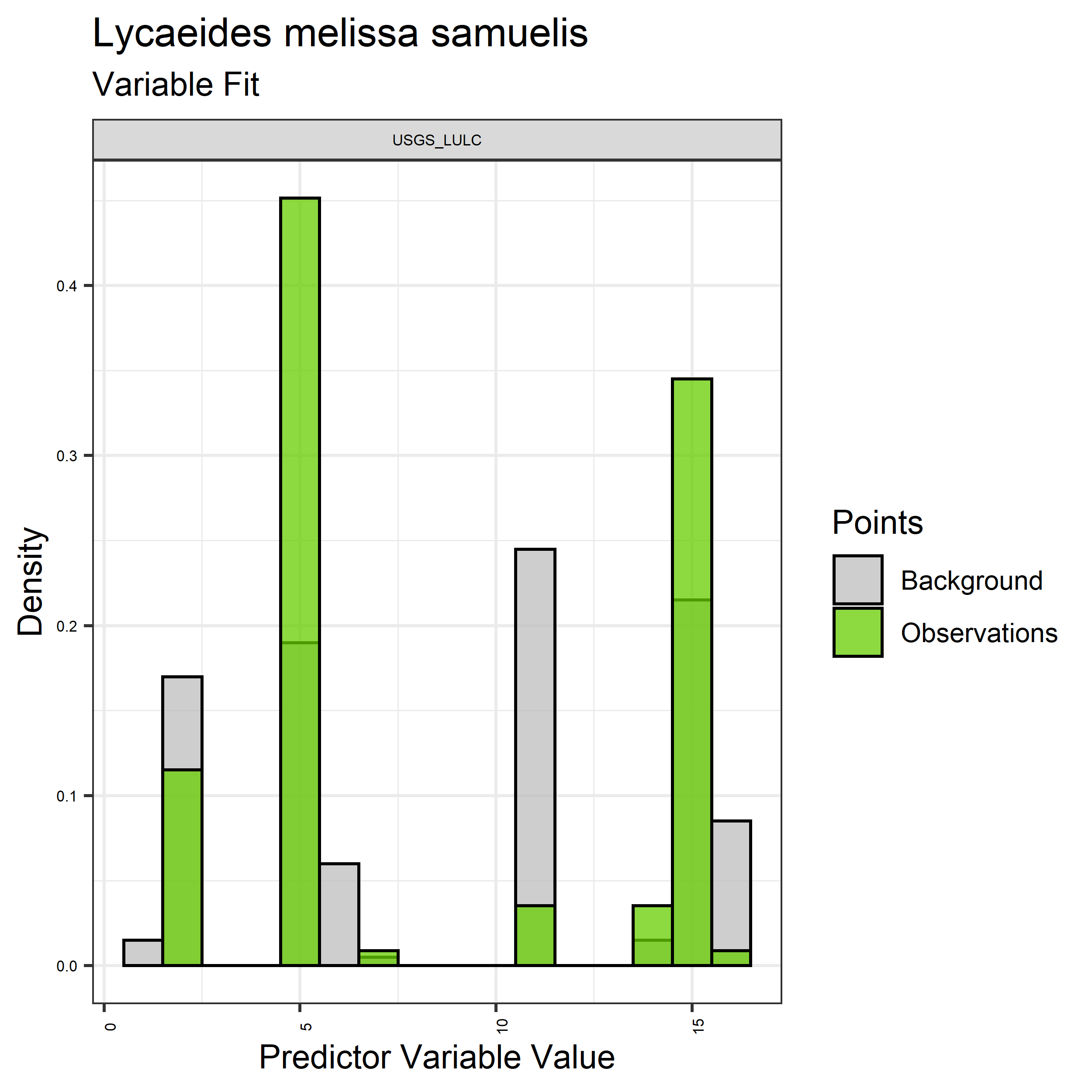
Figure 48. Sampling of discrete predictor variables retained in the best-fit Lycaeides melissa samuelis distribution models. Distribution of each variable at points of species occurrence (green) are contrasted with points sampled across the full modeled extent (gray).
|
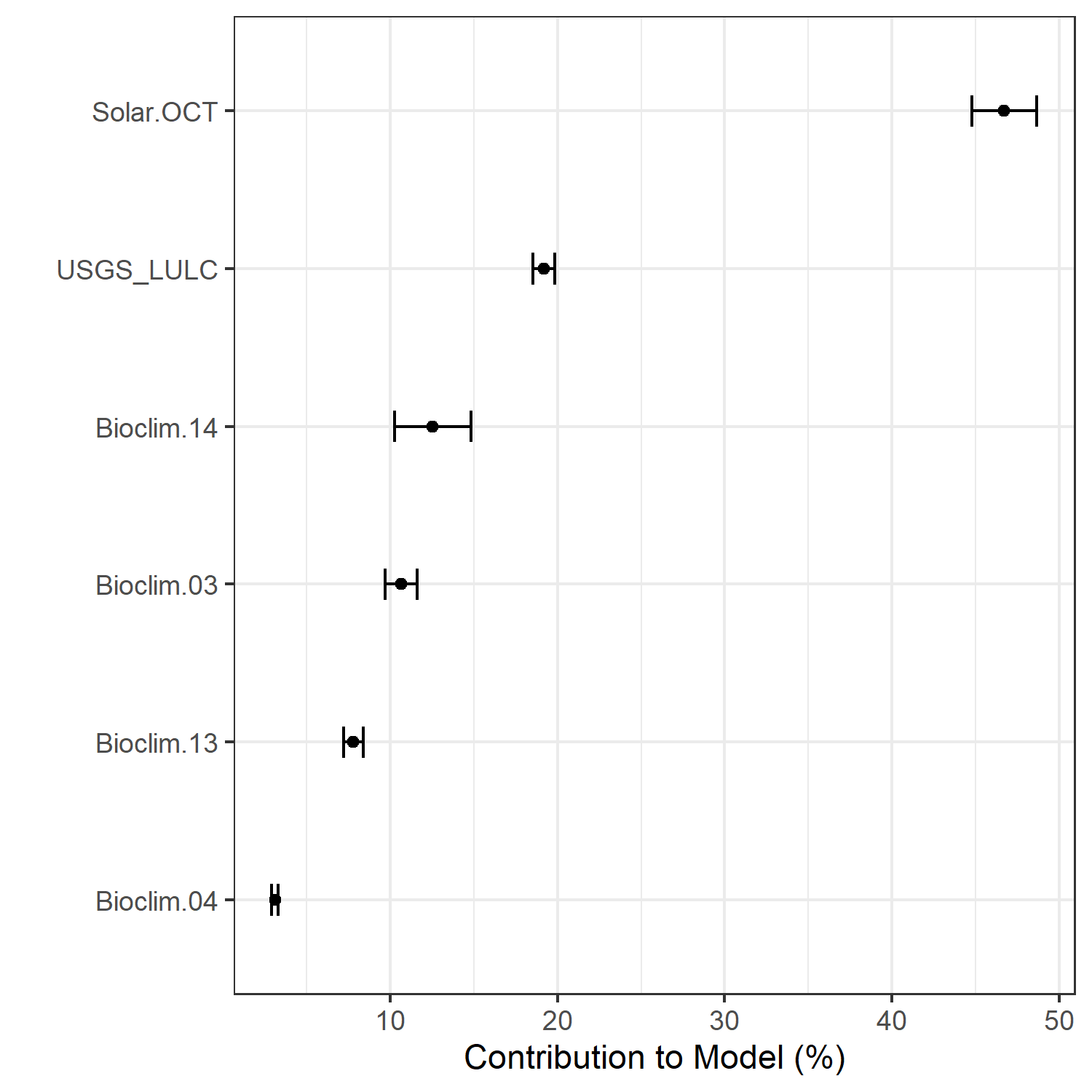
Figure 49. Percent contribution of each variable to best-fit species distribution models for Lycaeides melissa samuelis. Values sum to 1.0.
|
Table 24. Mean Area Under Curve (AUC) for five realizations of the best-fit SDM for Lycaeides melissa samuelis, calculated using 20% of species location records reserved for final evaluation.
| V1 |
V2 |
V3 |
V4 |
V5 |
mean |
sd |
| 0.959956 |
0.958142 |
0.958097 |
0.960752 |
0.959336 |
0.959257 |
0.001087 |
|
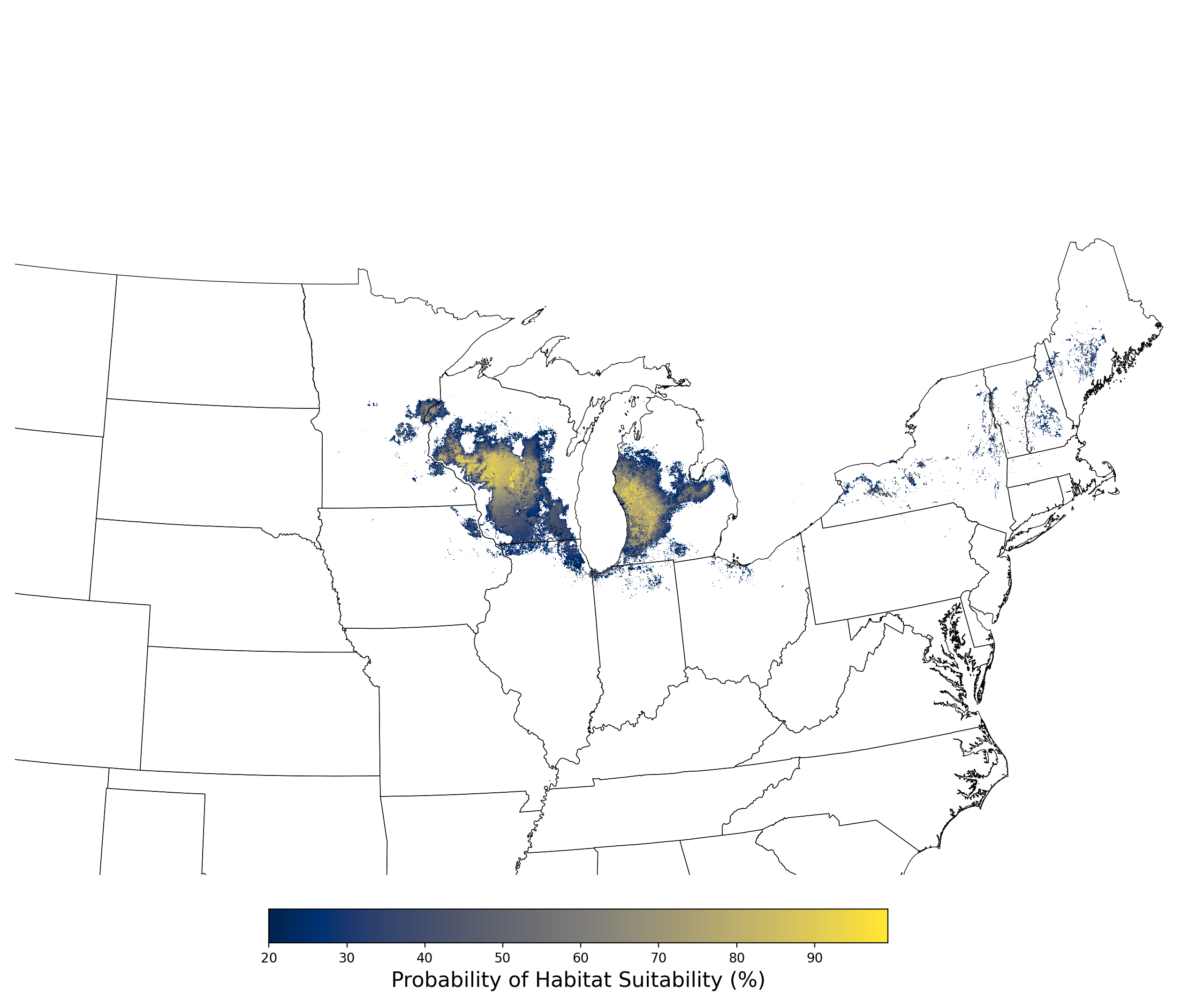
Figure 50. Final mean SDM output for Lycaeides melissa samuelis. |
2.2.8 Species Distribution Modeling Results for Neonympha mitchellii mitchellii
The species distribution modeling results consist of the following figures and tables:
- A table showing the SDM inputs (Table 25)
- A map showing the extent of SDM coverage (Figure 51)
- A graph showing the correlation between the predictor variable selected for evaluation (Figure 52)
- A graph of the model fit of each SDM iteration as measured by total Area Under Curve (AUC) where the curve is the Receiver Operating Curve, based on training data (Figure 53)
- A table showing the diagnostic statistics of the training data used in the final selected SDM iteration (Table 26)
- Graphs illustrating the predictor variable values sampled by the species observations and randomly selected background locations for continuous variables (Figure 54), and discrete variables (Figure 55)
- A graph showing the percent contribution of each predictor variable to the final selected SDM (Figure 56)
- A table showing the mean AUC for each of the five model runs that are averaged for the final selected SDM (Table 27)
- A map of the final averaged SDM (Figure 57)
Table 25. Input parameters for species distribution modeling of Neonympha mitchellii mitchellii.
| Number of predictors |
33 |
| Names of predictors |
Bioclim.01.tif, Bioclim.02.tif, Bioclim.03.tif, Bioclim.04.tif,
Bioclim.05.tif, Bioclim.06.tif, Bioclim.07.tif, Bioclim.08.tif,
Bioclim.09.tif, Bioclim.10.tif, Bioclim.11.tif, Bioclim.12.tif,
Bioclim.13.tif, Bioclim.14.tif, Bioclim.15.tif, Bioclim.16.tif,
Bioclim.17.tif, Bioclim.18.tif, Bioclim.19.tif, Elevation.tif,
Solar.APR.tif, Solar.AUG.tif, Solar.DEC.tif, Solar.FEB.tif,
Solar.JAN.tif, Solar.JUL.tif, Solar.JUN.tif, Solar.MAR.tif,
Solar.MAY.tif, Solar.NOV.tif, Solar.OCT.tif, Solar.SEP.tif,
USGS_LULC.tif |
| Predictor correlation threshold |
0.67 |
| Predictor contribution threshold |
1.0 |
| SDM threshold |
0.2 |
| Number of iterations conducted |
4 |
| Final SDM iteration number |
3 |
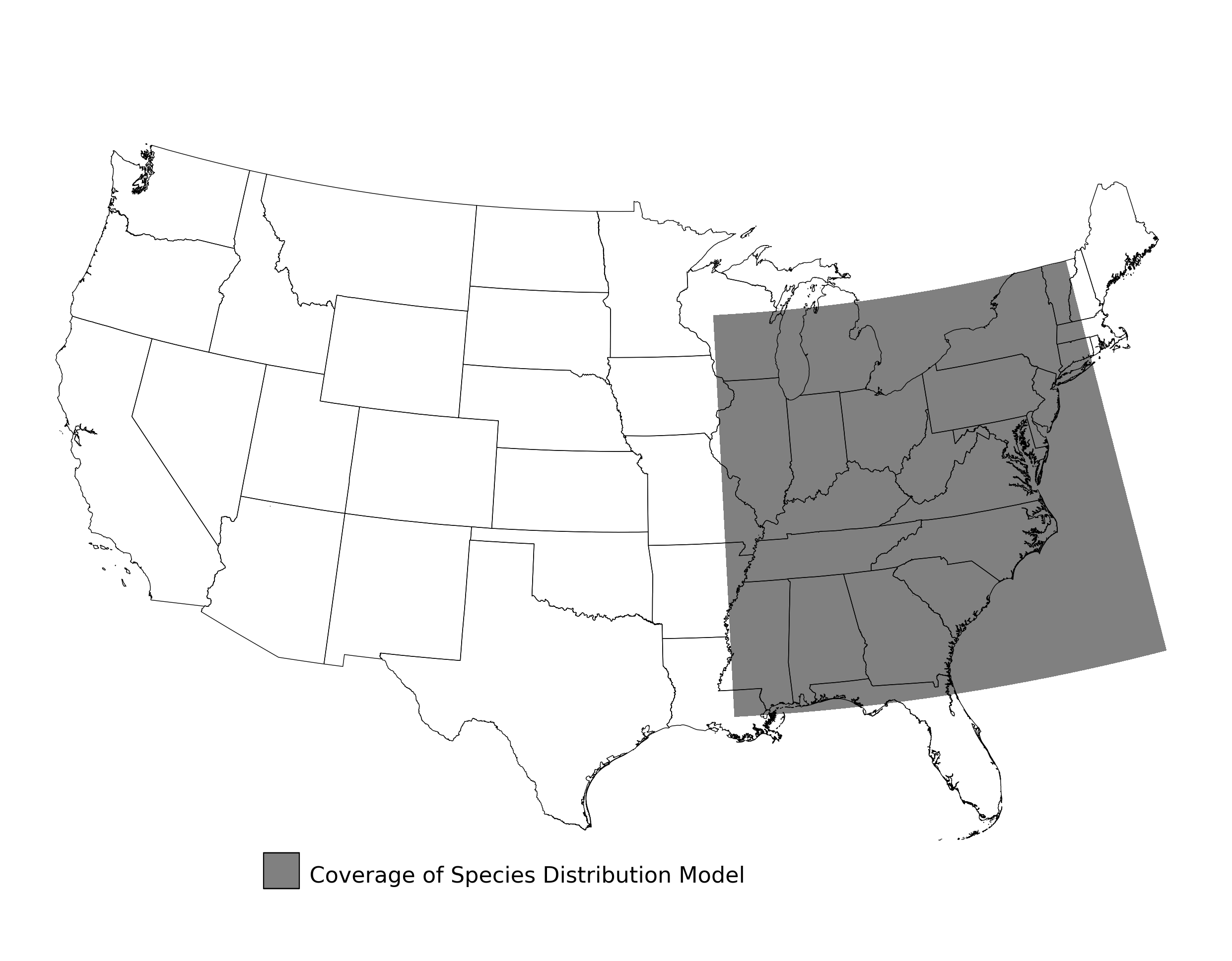
Figure 51. Extent of the species range modeled for Neonympha mitchellii mitchellii. Modeling extent is determined by buffering species location records in all directions by 3 degrees latitude/longitude.
|
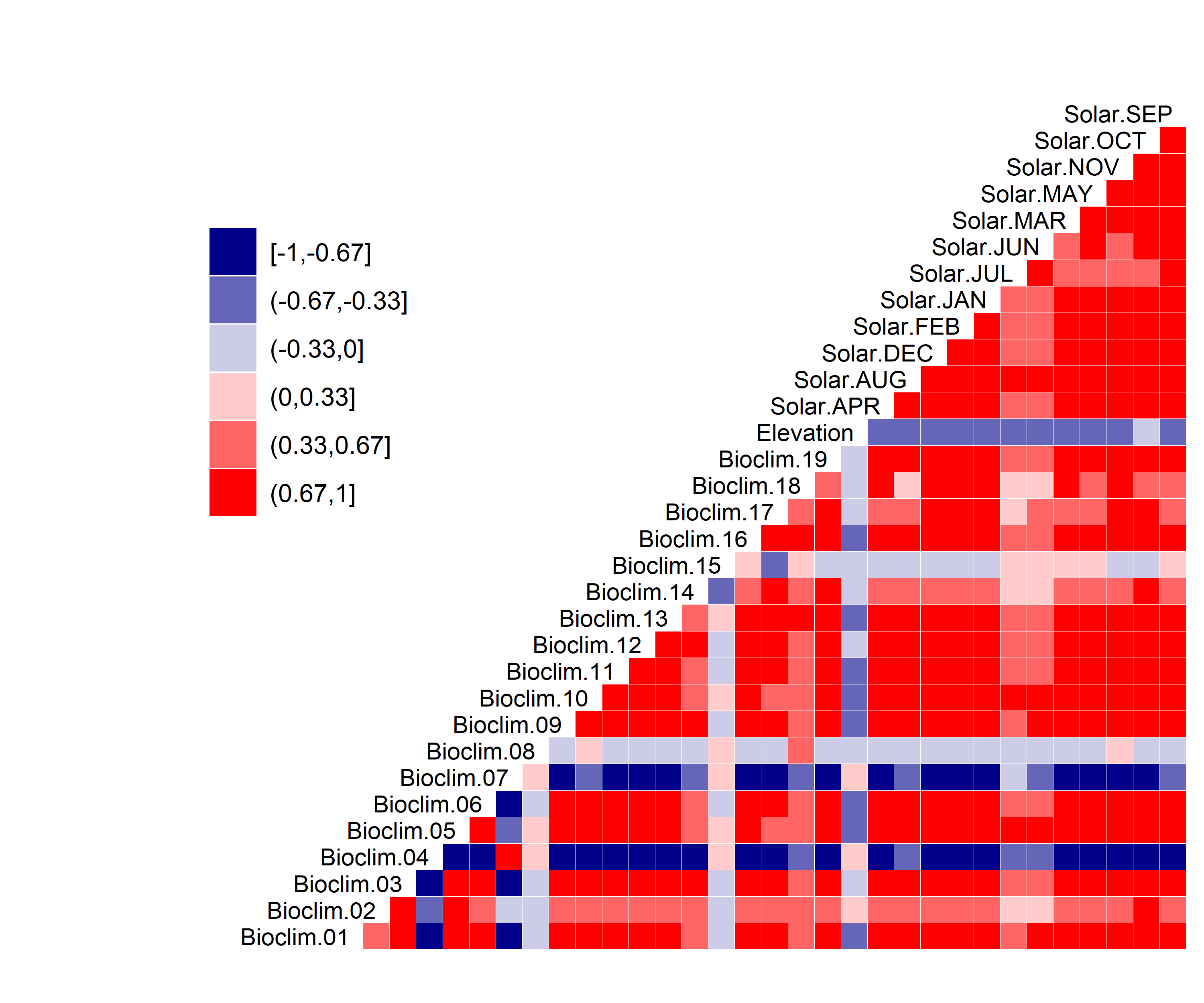
Figure 52. Correlation between SDM predictor variables for Neonympha mitchellii mitchellii.
|
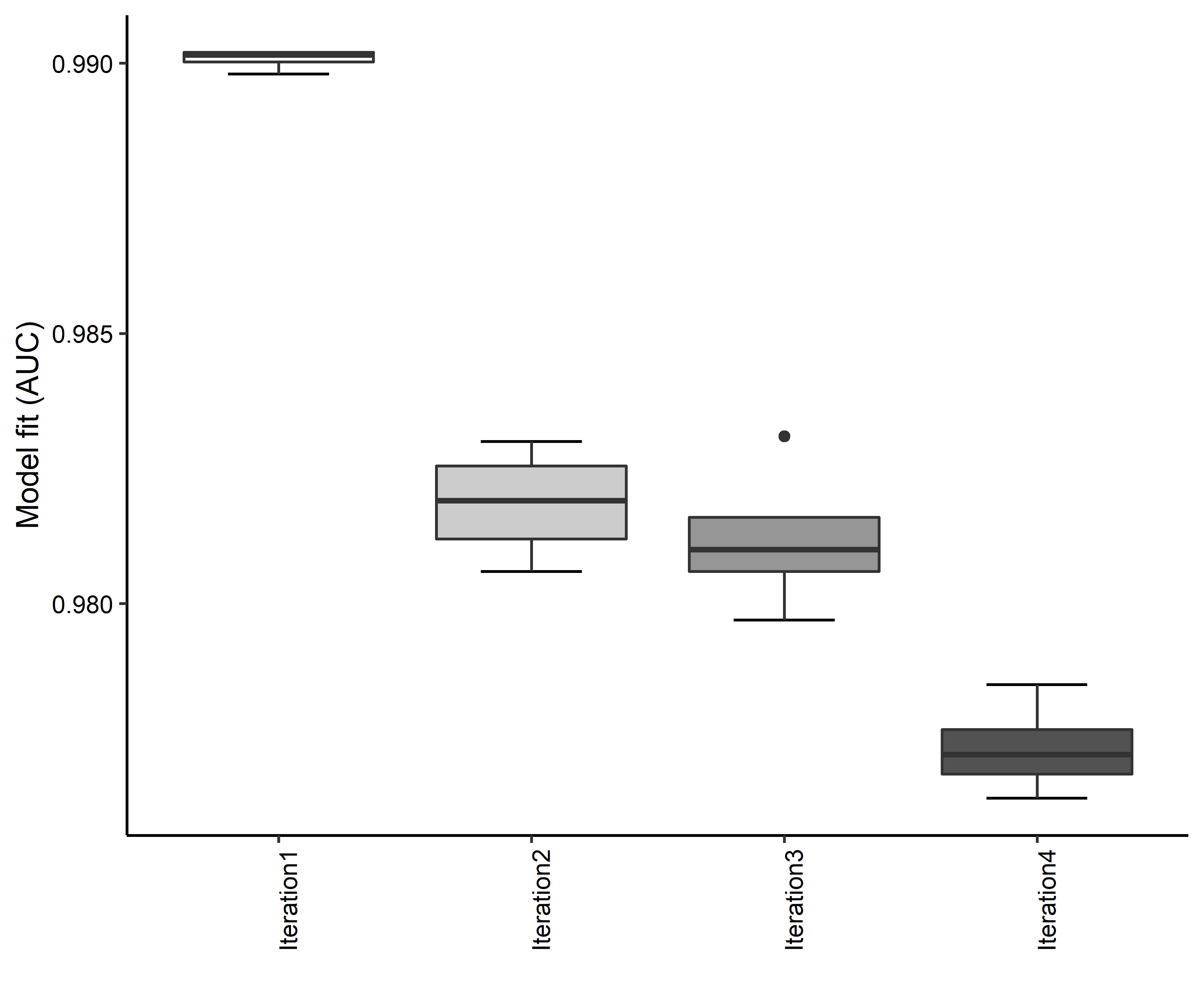
Figure 53. Boxplots of model fit for each iteration of Neonympha mitchellii mitchellii distribution modeling. Statistics are calculated using 80% of species location records reserved for model training.
|
Table 26. Diagnostic statistics of the training data used in SDM iteration #3 for Neonympha mitchellii mitchellii.
| Model Output |
Realization 1 |
Realization 2 |
Realization 3 |
Realization 4 |
Realization 5 |
Mean |
Standard Deviation |
| Number of training samples |
54.0000 |
54.0000 |
54.0000 |
54.0000 |
54.0000 |
54.00000 |
0.000000 |
| Regularized training gain |
1.5751 |
1.5979 |
1.5616 |
1.6768 |
1.5867 |
1.59962 |
0.045203 |
| Unregularized training gain |
2.5526 |
2.6164 |
2.5270 |
2.6868 |
2.5795 |
2.59246 |
0.062280 |
| Iterations |
500.0000 |
500.0000 |
500.0000 |
500.0000 |
500.0000 |
500.00000 |
0.000000 |
| Training AUC |
0.9795 |
0.9811 |
0.9797 |
0.9831 |
0.9809 |
0.98086 |
0.001438 |
| Number of background points |
10054.0000 |
10054.0000 |
10054.0000 |
10054.0000 |
10054.0000 |
10054.00000 |
0.000000 |
| Bioclim 02 contribution |
4.4859 |
5.0808 |
7.7277 |
6.6580 |
6.5506 |
6.10060 |
1.304597 |
| Bioclim 07 contribution |
5.1648 |
6.7296 |
6.7189 |
4.7950 |
8.3689 |
6.35544 |
1.429923 |
| Bioclim 08 contribution |
21.5801 |
17.9874 |
20.0154 |
16.8943 |
22.6428 |
19.82400 |
2.399083 |
| Bioclim 14 contribution |
11.6193 |
11.0470 |
11.6516 |
10.9312 |
9.5419 |
10.95820 |
0.856209 |
| Elevation contribution |
10.1556 |
11.1528 |
9.2736 |
9.6775 |
9.3130 |
9.91450 |
0.777856 |
| Solar SEP contribution |
34.9417 |
35.5125 |
34.4613 |
38.8091 |
33.2070 |
35.38632 |
2.093689 |
| USGS_LULC contribution |
12.0526 |
12.4900 |
10.1515 |
12.2348 |
10.3757 |
11.46092 |
1.106827 |
| Bioclim 02 permutation importance |
8.7765 |
12.6491 |
5.8203 |
8.3262 |
9.6957 |
9.05356 |
2.469820 |
| Bioclim 07 permutation importance |
9.1677 |
13.4480 |
9.7995 |
5.8807 |
12.9483 |
10.24884 |
3.081117 |
| Bioclim 08 permutation importance |
18.7134 |
19.0139 |
28.2465 |
21.4540 |
27.1235 |
22.91026 |
4.503965 |
| Bioclim 14 permutation importance |
4.4238 |
4.4113 |
6.8903 |
7.2922 |
5.6910 |
5.74172 |
1.344687 |
| Elevation permutation importance |
19.8469 |
17.3427 |
13.1991 |
19.8486 |
12.0982 |
16.46710 |
3.653470 |
| Solar SEP permutation importance |
31.2300 |
25.2650 |
26.7832 |
29.8114 |
27.2418 |
28.06628 |
2.409761 |
| USGS_LULC permutation importance |
7.8418 |
7.8701 |
9.2612 |
7.3870 |
5.2015 |
7.51232 |
1.470607 |
| Entropy |
7.6446 |
7.6176 |
7.6820 |
7.5566 |
7.6393 |
7.62802 |
0.046166 |
| Prevalence average probability of presence over background sites |
0.1187 |
0.1154 |
0.1228 |
0.1086 |
0.1181 |
0.11672 |
0.005255 |
| Fixed cumulative value 1 cumulative threshold |
1.0000 |
1.0000 |
1.0000 |
1.0000 |
1.0000 |
1.00000 |
0.000000 |
| Fixed cumulative value 1 Cloglog threshold |
0.0178 |
0.0177 |
0.0191 |
0.0166 |
0.0182 |
0.01788 |
0.000904 |
| Fixed cumulative value 1 area |
0.5658 |
0.5588 |
0.5799 |
0.5604 |
0.5650 |
0.56598 |
0.008328 |
| Fixed cumulative value 1 training omission |
0.0000 |
0.0000 |
0.0000 |
0.0000 |
0.0000 |
0.00000 |
0.000000 |
| Fixed cumulative value 5 cumulative threshold |
5.0000 |
5.0000 |
5.0000 |
5.0000 |
5.0000 |
5.00000 |
0.000000 |
| Fixed cumulative value 5 Cloglog threshold |
0.0724 |
0.0679 |
0.0710 |
0.0633 |
0.0709 |
0.06910 |
0.003634 |
| Fixed cumulative value 5 area |
0.3557 |
0.3489 |
0.3655 |
0.3488 |
0.3553 |
0.35484 |
0.006826 |
| Fixed cumulative value 5 training omission |
0.0000 |
0.0000 |
0.0000 |
0.0000 |
0.0000 |
0.00000 |
0.000000 |
| Fixed cumulative value 10 cumulative threshold |
10.0000 |
10.0000 |
10.0000 |
10.0000 |
10.0000 |
10.00000 |
0.000000 |
| Fixed cumulative value 10 Cloglog threshold |
0.1292 |
0.1270 |
0.1292 |
0.1179 |
0.1294 |
0.12654 |
0.004929 |
| Fixed cumulative value 10 area |
0.2560 |
0.2476 |
0.2616 |
0.2447 |
0.2547 |
0.25292 |
0.006780 |
| Fixed cumulative value 10 training omission |
0.0000 |
0.0000 |
0.0000 |
0.0000 |
0.0000 |
0.00000 |
0.000000 |
| Minimum training presence cumulative threshold |
28.7228 |
26.6832 |
30.5513 |
30.4918 |
27.9033 |
28.87048 |
1.672967 |
| Minimum training presence Cloglog threshold |
0.3693 |
0.3487 |
0.4150 |
0.3904 |
0.3657 |
0.37782 |
0.025535 |
| Minimum training presence area |
0.1043 |
0.1082 |
0.0974 |
0.0880 |
0.1062 |
0.10082 |
0.008240 |
| Minimum training presence training omission |
0.0000 |
0.0000 |
0.0000 |
0.0000 |
0.0000 |
0.00000 |
0.000000 |
| X10 percentile training presence cumulative threshold |
43.6113 |
48.6223 |
45.8221 |
49.8222 |
48.1993 |
47.21544 |
2.483629 |
| X10 percentile training presence Cloglog threshold |
0.5664 |
0.6491 |
0.6103 |
0.6503 |
0.6250 |
0.62022 |
0.034484 |
| X10 percentile training presence area |
0.0540 |
0.0415 |
0.0501 |
0.0367 |
0.0432 |
0.04510 |
0.006916 |
| X10 percentile training presence training omission |
0.0926 |
0.0926 |
0.0926 |
0.0926 |
0.0926 |
0.09260 |
0.000000 |
| Equal training sensitivity and specificity cumulative threshold |
40.3807 |
42.1299 |
43.5024 |
42.1420 |
42.8327 |
42.19754 |
1.163471 |
| Equal training sensitivity and specificity Cloglog threshold |
0.5218 |
0.5649 |
0.5751 |
0.5464 |
0.5572 |
0.55308 |
0.020400 |
| Equal training sensitivity and specificity area |
0.0626 |
0.0556 |
0.0556 |
0.0528 |
0.0556 |
0.05644 |
0.003651 |
| Equal training sensitivity and specificity training omission |
0.0556 |
0.0556 |
0.0556 |
0.0556 |
0.0556 |
0.05560 |
0.000000 |
| Maximum training sensitivity plus specificity cumulative threshold |
36.4006 |
35.5245 |
39.5715 |
37.8808 |
38.8445 |
37.64438 |
1.677115 |
| Maximum training sensitivity plus specificity Cloglog threshold |
0.4694 |
0.4709 |
0.5254 |
0.4910 |
0.5069 |
0.49272 |
0.023937 |
| Maximum training sensitivity plus specificity area |
0.0747 |
0.0740 |
0.0662 |
0.0640 |
0.0665 |
0.06908 |
0.004913 |
| Maximum training sensitivity plus specificity training omission |
0.0185 |
0.0185 |
0.0185 |
0.0185 |
0.0185 |
0.01850 |
0.000000 |
| Balance training omission predicted area and threshold value cumulative threshold |
5.5906 |
5.8095 |
5.9125 |
5.9538 |
5.6340 |
5.78008 |
0.162651 |
| Balance training omission predicted area and threshold value Cloglog threshold |
0.0797 |
0.0777 |
0.0827 |
0.0733 |
0.0794 |
0.07856 |
0.003448 |
| Balance training omission predicted area and threshold value area |
0.3403 |
0.3274 |
0.3410 |
0.3233 |
0.3384 |
0.33408 |
0.008156 |
| Balance training omission predicted area and threshold value training omission |
0.0000 |
0.0000 |
0.0000 |
0.0000 |
0.0000 |
0.00000 |
0.000000 |
| Equate entropy of thresholded and original distributions cumulative threshold |
13.7283 |
13.5291 |
13.4002 |
14.3444 |
13.7369 |
13.74778 |
0.362314 |
| Equate entropy of thresholded and original distributions Cloglog threshold |
0.1694 |
0.1674 |
0.1671 |
0.1672 |
0.1695 |
0.16812 |
0.001219 |
| Equate entropy of thresholded and original distributions area |
0.2078 |
0.2022 |
0.2157 |
0.1903 |
0.2067 |
0.20454 |
0.009329 |
| Equate entropy of thresholded and original distributions training omission |
0.0000 |
0.0000 |
0.0000 |
0.0000 |
0.0000 |
0.00000 |
0.000000 |
|
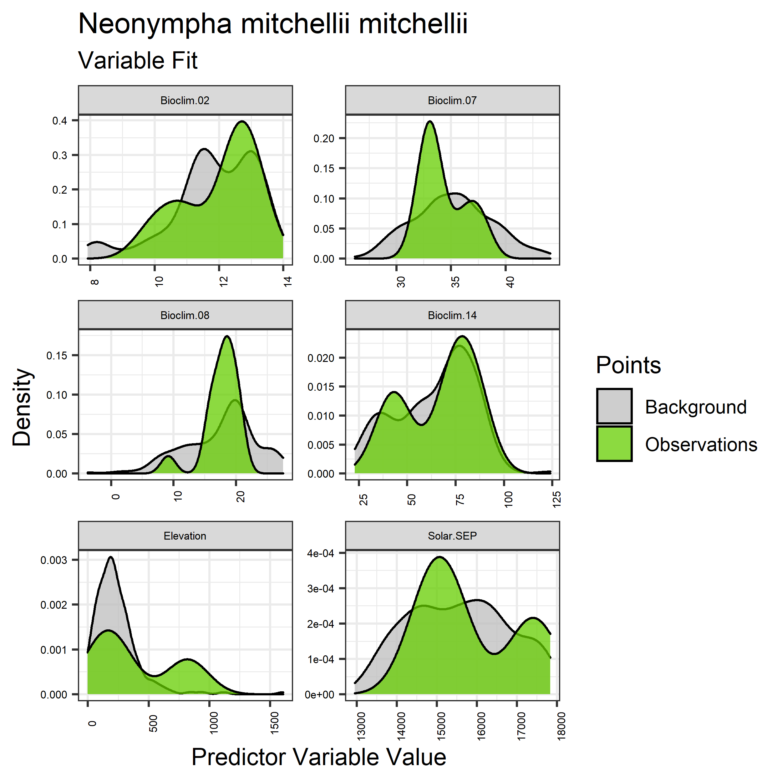
Figure 54. Sampling of continuous predictor variables retained in the best-fit Neonympha mitchellii mitchellii distribution models. Distribution of each variable at points of species occurrence (green) are contrasted with points sampled across the full modeled extent (gray).
|
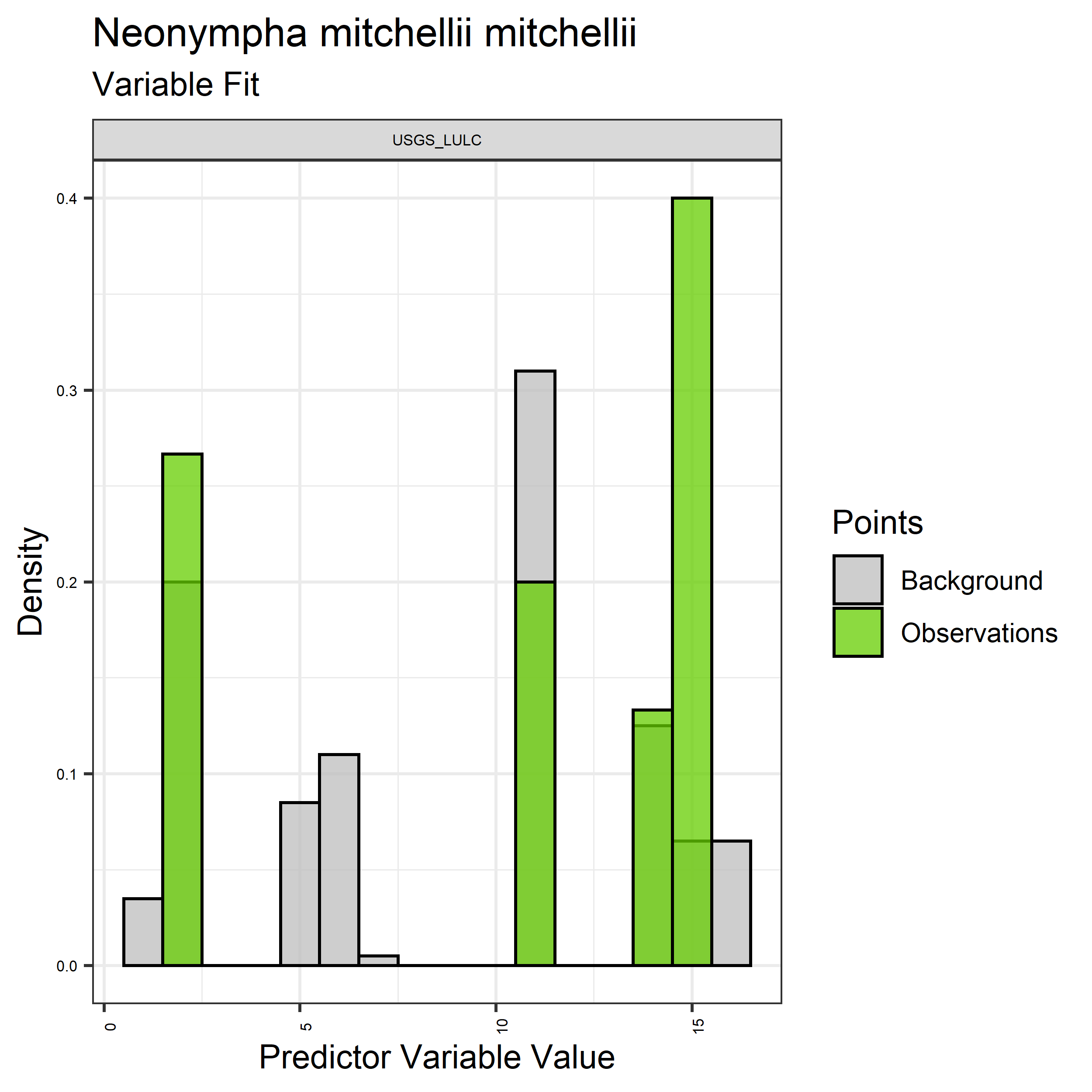
Figure 55. Sampling of discrete predictor variables retained in the best-fit Neonympha mitchellii mitchellii distribution models. Distribution of each variable at points of species occurrence (green) are contrasted with points sampled across the full modeled extent.
|
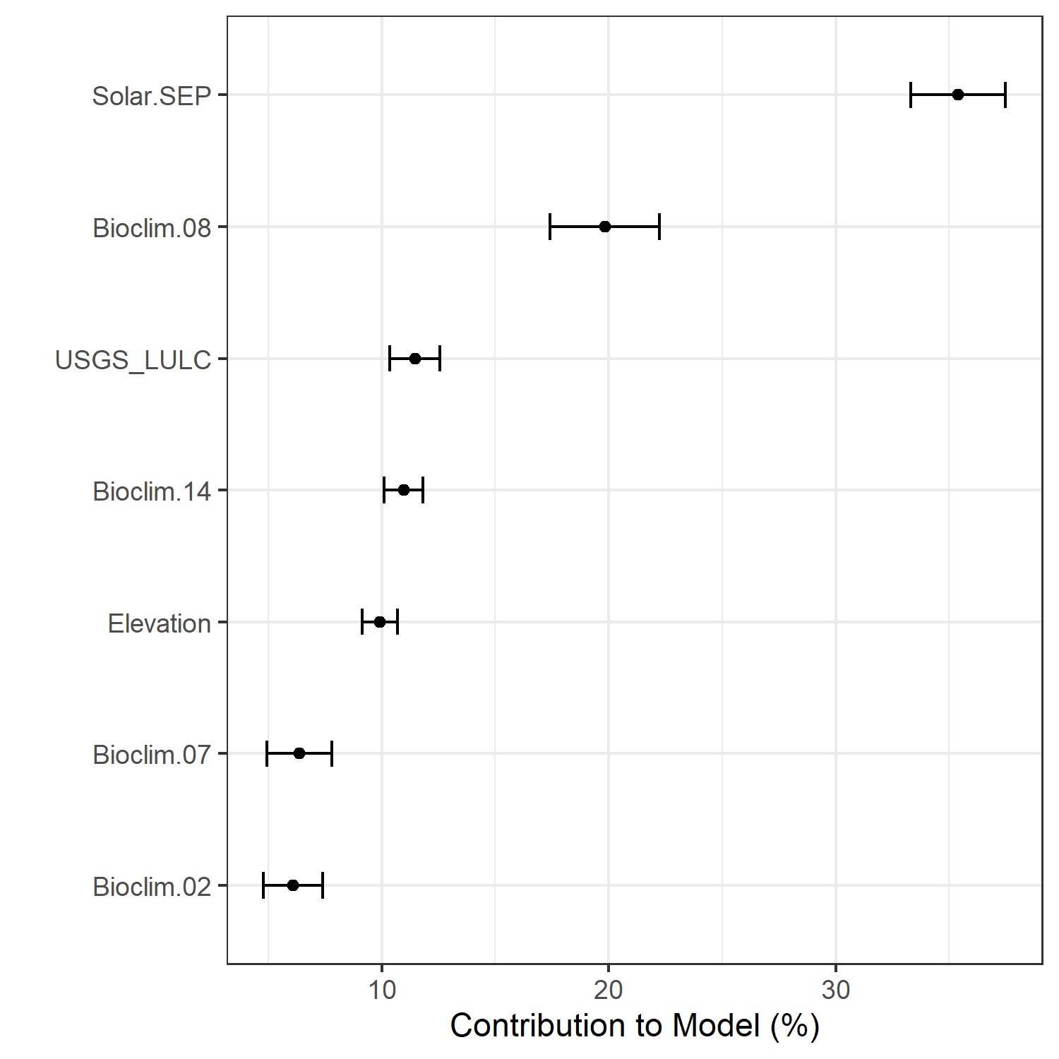
Figure 56. Percent contribution of each variable to best-fit species distribution models for Neonympha mitchellii mitchellii. Values sum to 1.0.
|
Table 27. Mean Area Under Curve (AUC) for five realizations of the best-fit SDM for Neonympha mitchellii mitchellii, calculated using 20% of species location records reserved for final evaluation.
| V1 |
V2 |
V3 |
V4 |
V5 |
mean |
sd |
| 0.968333 |
0.973 |
0.973667 |
0.974333 |
0.972 |
0.972267 |
0.001117 |
|
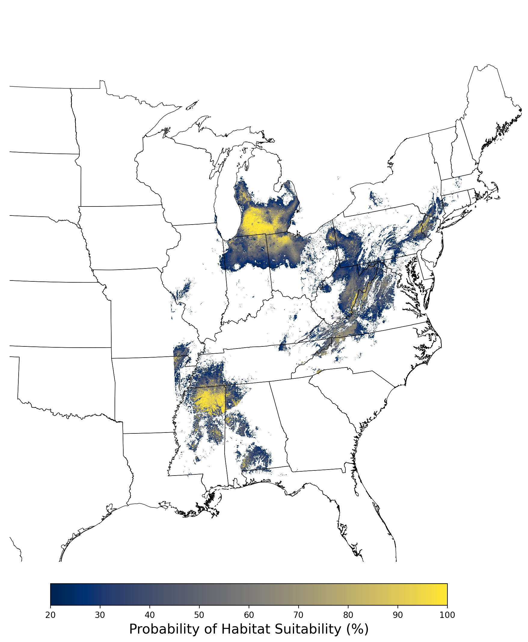
Figure 57. Final mean SDM output for Neonympha mitchellii mitchellii. |
2.2.9 Species Distribution Modeling Results for Pedicularis furbishiae
The species distribution modeling results consist of the following figures and tables:
- A table showing the SDM inputs (Table 28)
- A map showing the extent of SDM coverage (Figure 58)
- A graph showing the correlation between the predictor variable selected for evaluation (Figure 59)
- A graph of the model fit of each SDM iteration as measured by total Area Under Curve (AUC) where the curve is the Receiver Operating Curve, based on training data (Figure 60)
- A table showing the diagnostic statistics of the training data used in the final selected SDM iteration (Table 29)
- Graphs illustrating the predictor variable values sampled by the species observations and randomly selected background locations for continuous variables (Figure 61), and discrete variables (Figure 62)
- A graph showing the percent contribution of each predictor variable to the final selected SDM (Figure 63)
- A table showing the mean AUC for each of the five model runs that are averaged for the final selected SDM (Table 30)
- A map of the final averaged SDM (Figure 64)
Table 28. Input parameters for species distribution modeling of Pedicularis furbishiae.
| Number of predictors |
33 |
| Names of predictors |
Bioclim.01.tif, Bioclim.02.tif, Bioclim.03.tif, Bioclim.04.tif,
Bioclim.05.tif, Bioclim.06.tif, Bioclim.07.tif, Bioclim.08.tif,
Bioclim.09.tif, Bioclim.10.tif, Bioclim.11.tif, Bioclim.12.tif,
Bioclim.13.tif, Bioclim.14.tif, Bioclim.15.tif, Bioclim.16.tif,
Bioclim.17.tif, Bioclim.18.tif, Bioclim.19.tif, Elevation.tif,
Solar.APR.tif, Solar.AUG.tif, Solar.DEC.tif, Solar.FEB.tif,
Solar.JAN.tif, Solar.JUL.tif, Solar.JUN.tif, Solar.MAR.tif,
Solar.MAY.tif, Solar.NOV.tif, Solar.OCT.tif, Solar.SEP.tif,
USGS_LULC.tif |
| Predictor correlation threshold |
0.67 |
| Predictor contribution threshold |
1.0 |
| SDM threshold |
0.2 |
| Number of iterations conducted |
4 |
| Final SDM iteration number |
3 |
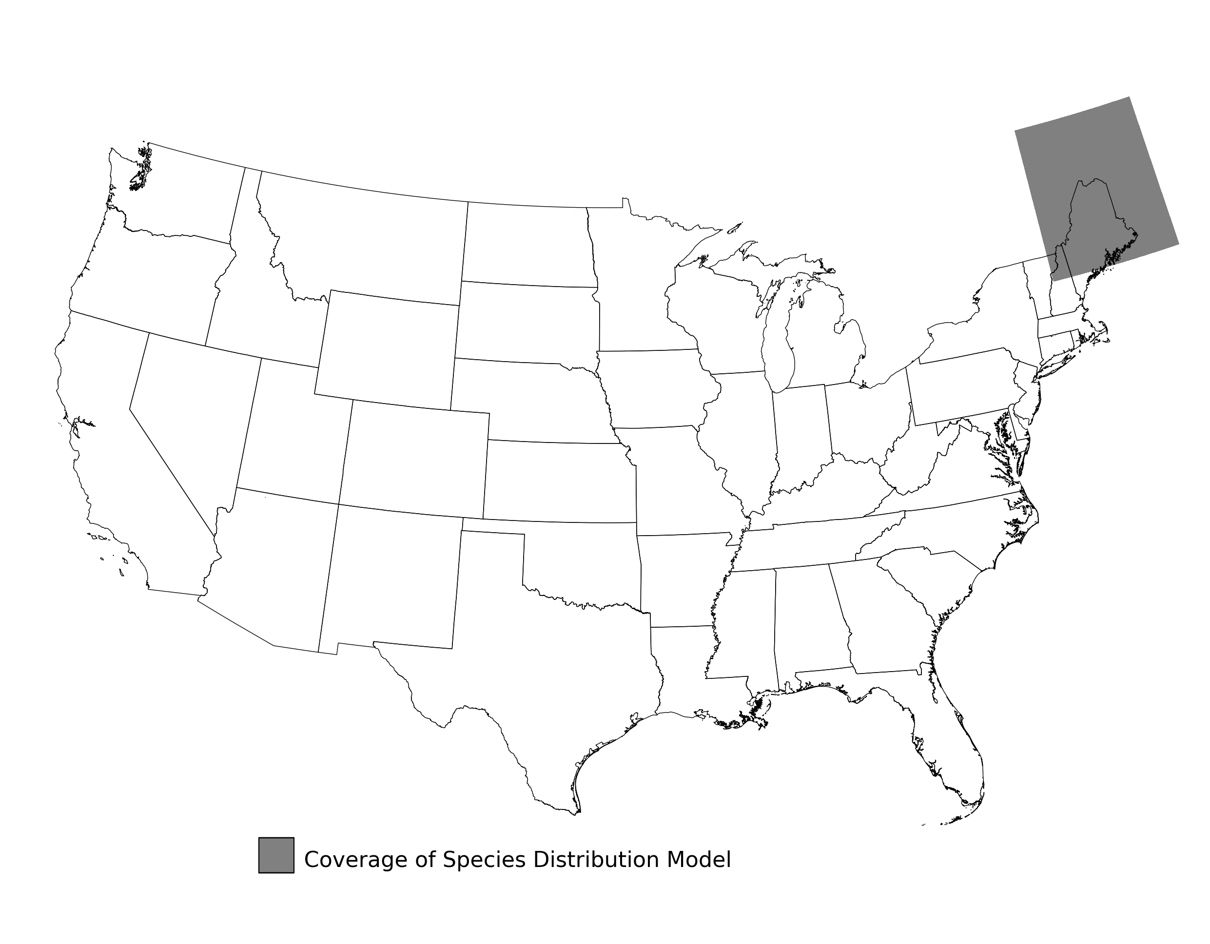
Figure 58. Extent of the species range modeled for Pedicularis furbishiae. Modeling extent is determined by buffering species location records in all directions by 3 degrees latitude/longitude.
|
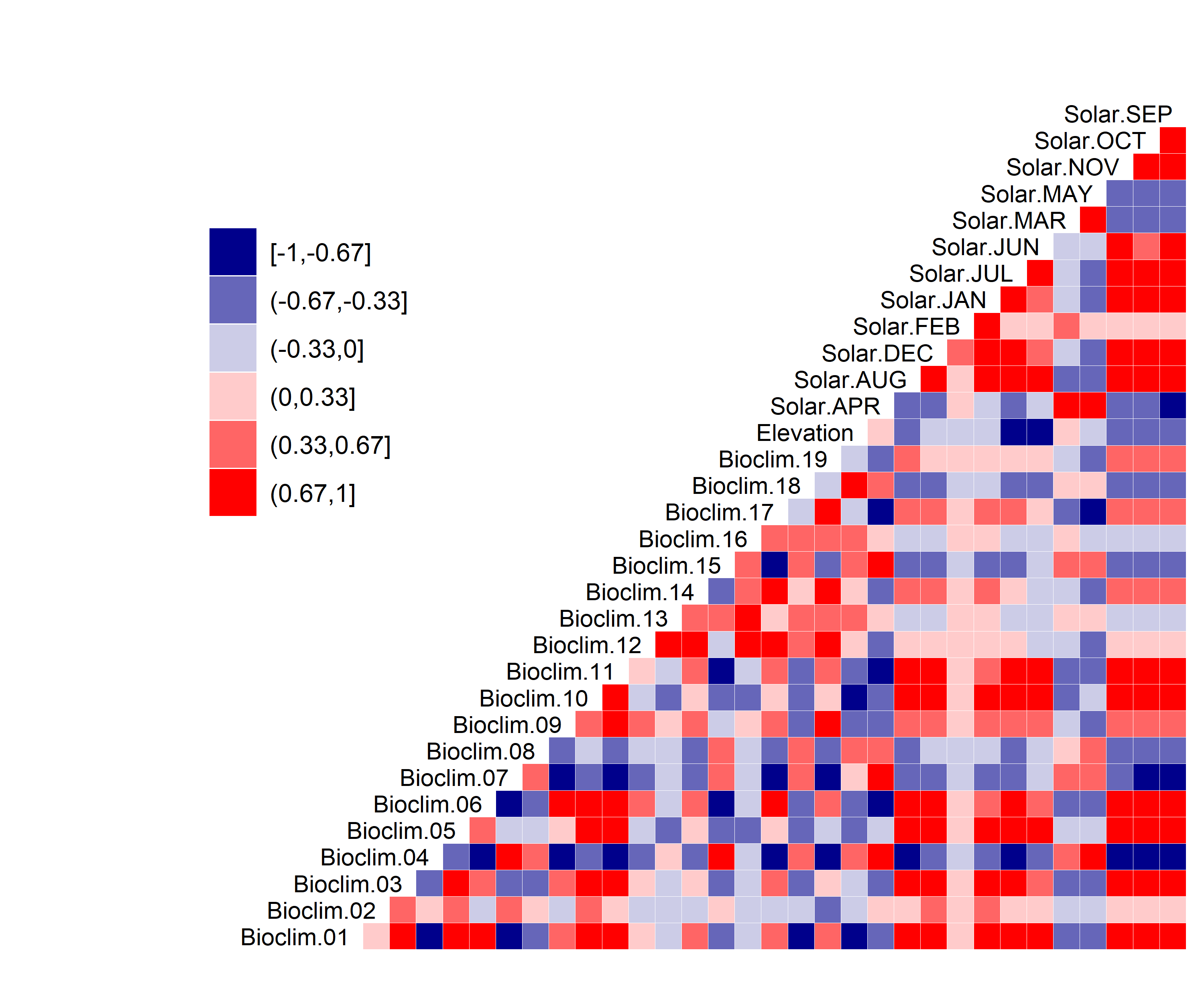
Figure 59. Correlation between SDM predictor variables for Pedicularis furbishiae.
|
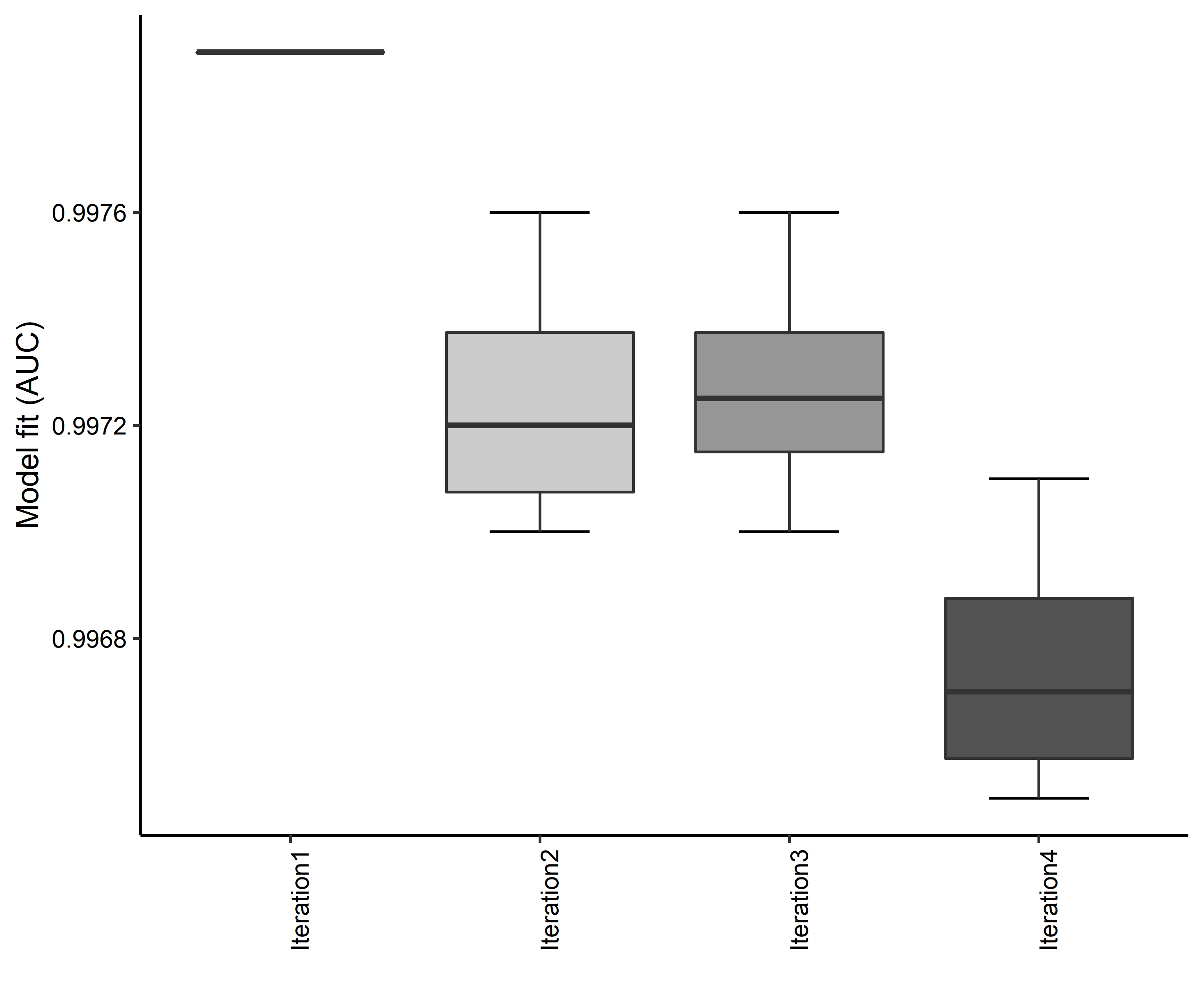
Figure 60. Boxplots of model fit for each iteration of Pedicularis furbishiae distribution modeling. Statistics are calculated using 80% of species location records reserved for model training.
|
Table 29. Diagnostic statistics of the training data used in SDM iteration #3 for Pedicularis furbishiae.
| Model Output |
Realization 1 |
Realization 2 |
Realization 3 |
Realization 4 |
Realization 5 |
Mean |
Standard Deviation |
| Number of training samples |
37.0000 |
37.0000 |
37.0000 |
37.0000 |
37.0000 |
37.00000 |
0.000000 |
| Regularized training gain |
3.9154 |
3.8182 |
3.9576 |
3.9266 |
3.9027 |
3.90410 |
0.052146 |
| Unregularized training gain |
4.6747 |
4.5469 |
4.7330 |
4.6593 |
4.6551 |
4.65380 |
0.067396 |
| Iterations |
500.0000 |
500.0000 |
500.0000 |
500.0000 |
500.0000 |
500.00000 |
0.000000 |
| Training AUC |
0.9975 |
0.9970 |
0.9976 |
0.9972 |
0.9973 |
0.99732 |
0.000239 |
| Number of background points |
10037.0000 |
10037.0000 |
10037.0000 |
10037.0000 |
10037.0000 |
10037.00000 |
0.000000 |
| Bioclim 03 contribution |
38.7168 |
38.4246 |
39.6503 |
37.9631 |
37.8007 |
38.51110 |
0.733577 |
| Bioclim 08 contribution |
5.2683 |
6.9337 |
5.1715 |
5.0426 |
6.3428 |
5.75178 |
0.839591 |
| Bioclim 12 contribution |
25.2815 |
28.4996 |
26.5655 |
28.1025 |
27.7879 |
27.24740 |
1.315398 |
| Elevation contribution |
7.4124 |
7.2365 |
6.7517 |
6.8298 |
7.5038 |
7.14684 |
0.340085 |
| Solar APR contribution |
9.8783 |
7.0080 |
8.5466 |
9.6225 |
6.3273 |
8.27654 |
1.569945 |
| Solar FEB contribution |
8.9270 |
7.8673 |
8.5454 |
7.7156 |
9.2638 |
8.46382 |
0.666489 |
| USGS_LULC contribution |
4.5156 |
4.0303 |
4.7690 |
4.7239 |
4.9737 |
4.60250 |
0.358892 |
| Bioclim 03 permutation importance |
27.0399 |
33.5996 |
25.5100 |
26.2156 |
33.0559 |
29.08420 |
3.916190 |
| Bioclim 08 permutation importance |
2.1973 |
3.2323 |
4.7594 |
0.8726 |
5.5381 |
3.31994 |
1.887442 |
| Bioclim 12 permutation importance |
35.5109 |
31.3718 |
41.4845 |
35.2217 |
23.7286 |
33.46350 |
6.533817 |
| Elevation permutation importance |
20.2944 |
18.9433 |
10.4021 |
23.9828 |
24.5203 |
19.62858 |
5.677346 |
| Solar APR permutation importance |
10.5660 |
9.2995 |
14.1041 |
10.2721 |
6.2464 |
10.09762 |
2.818271 |
| Solar FEB permutation importance |
3.9712 |
3.4270 |
3.4149 |
3.1870 |
6.3992 |
4.07986 |
1.328226 |
| USGS_LULC permutation importance |
0.4202 |
0.1264 |
0.3250 |
0.2482 |
0.5116 |
0.32628 |
0.149344 |
| Entropy |
5.3075 |
5.3994 |
5.2713 |
5.2915 |
5.3316 |
5.32026 |
0.049444 |
| Prevalence average probability of presence over background sites |
0.0109 |
0.0119 |
0.0105 |
0.0106 |
0.0111 |
0.01100 |
0.000557 |
| Fixed cumulative value 1 cumulative threshold |
1.0000 |
1.0000 |
1.0000 |
1.0000 |
1.0000 |
1.00000 |
0.000000 |
| Fixed cumulative value 1 Cloglog threshold |
0.0045 |
0.0050 |
0.0045 |
0.0044 |
0.0049 |
0.00466 |
0.000270 |
| Fixed cumulative value 1 area |
0.1057 |
0.1070 |
0.1004 |
0.1065 |
0.1054 |
0.10500 |
0.002649 |
| Fixed cumulative value 1 training omission |
0.0000 |
0.0000 |
0.0000 |
0.0000 |
0.0000 |
0.00000 |
0.000000 |
| Fixed cumulative value 5 cumulative threshold |
5.0000 |
5.0000 |
5.0000 |
5.0000 |
5.0000 |
5.00000 |
0.000000 |
| Fixed cumulative value 5 Cloglog threshold |
0.0327 |
0.0349 |
0.0333 |
0.0309 |
0.0340 |
0.03316 |
0.001506 |
| Fixed cumulative value 5 area |
0.0422 |
0.0436 |
0.0403 |
0.0419 |
0.0429 |
0.04218 |
0.001240 |
| Fixed cumulative value 5 training omission |
0.0000 |
0.0000 |
0.0000 |
0.0000 |
0.0000 |
0.00000 |
0.000000 |
| Fixed cumulative value 10 cumulative threshold |
10.0000 |
10.0000 |
10.0000 |
10.0000 |
10.0000 |
10.00000 |
0.000000 |
| Fixed cumulative value 10 Cloglog threshold |
0.0893 |
0.1032 |
0.0916 |
0.0848 |
0.0878 |
0.09134 |
0.007074 |
| Fixed cumulative value 10 area |
0.0241 |
0.0261 |
0.0230 |
0.0232 |
0.0247 |
0.02422 |
0.001256 |
| Fixed cumulative value 10 training omission |
0.0000 |
0.0000 |
0.0000 |
0.0000 |
0.0000 |
0.00000 |
0.000000 |
| Minimum training presence cumulative threshold |
35.9764 |
23.1208 |
32.8803 |
22.8267 |
29.3250 |
28.82584 |
5.838567 |
| Minimum training presence Cloglog threshold |
0.5409 |
0.2851 |
0.5177 |
0.3375 |
0.4373 |
0.42370 |
0.111127 |
| Minimum training presence area |
0.0057 |
0.0112 |
0.0060 |
0.0097 |
0.0074 |
0.00800 |
0.002386 |
| Minimum training presence training omission |
0.0000 |
0.0000 |
0.0000 |
0.0000 |
0.0000 |
0.00000 |
0.000000 |
| X10 percentile training presence cumulative threshold |
39.1479 |
37.1916 |
39.5831 |
37.8425 |
37.9869 |
38.35040 |
0.985960 |
| X10 percentile training presence Cloglog threshold |
0.6275 |
0.5964 |
0.6698 |
0.6628 |
0.6363 |
0.63856 |
0.029447 |
| X10 percentile training presence area |
0.0050 |
0.0057 |
0.0047 |
0.0049 |
0.0052 |
0.00510 |
0.000381 |
| X10 percentile training presence training omission |
0.0811 |
0.0811 |
0.0811 |
0.0811 |
0.0811 |
0.08110 |
0.000000 |
| Equal training sensitivity and specificity cumulative threshold |
35.9764 |
23.1208 |
32.8803 |
22.8267 |
29.3250 |
28.82584 |
5.838567 |
| Equal training sensitivity and specificity Cloglog threshold |
0.5409 |
0.2851 |
0.5177 |
0.3375 |
0.4373 |
0.42370 |
0.111127 |
| Equal training sensitivity and specificity area |
0.0057 |
0.0112 |
0.0060 |
0.0097 |
0.0074 |
0.00800 |
0.002386 |
| Equal training sensitivity and specificity training omission |
0.0000 |
0.0000 |
0.0000 |
0.0000 |
0.0000 |
0.00000 |
0.000000 |
| Maximum training sensitivity plus specificity cumulative threshold |
35.9764 |
23.1208 |
32.8803 |
22.8267 |
29.3250 |
28.82584 |
5.838567 |
| Maximum training sensitivity plus specificity Cloglog threshold |
0.5409 |
0.2851 |
0.5177 |
0.3375 |
0.4373 |
0.42370 |
0.111127 |
| Maximum training sensitivity plus specificity area |
0.0057 |
0.0112 |
0.0060 |
0.0097 |
0.0074 |
0.00800 |
0.002386 |
| Maximum training sensitivity plus specificity training omission |
0.0000 |
0.0000 |
0.0000 |
0.0000 |
0.0000 |
0.00000 |
0.000000 |
| Balance training omission predicted area and threshold value cumulative threshold |
1.6947 |
1.6920 |
1.6321 |
1.7014 |
1.6545 |
1.67494 |
0.030144 |
| Balance training omission predicted area and threshold value Cloglog threshold |
0.0080 |
0.0087 |
0.0077 |
0.0078 |
0.0082 |
0.00808 |
0.000396 |
| Balance training omission predicted area and threshold value area |
0.0824 |
0.0844 |
0.0799 |
0.0834 |
0.0841 |
0.08284 |
0.001815 |
| Balance training omission predicted area and threshold value training omission |
0.0000 |
0.0000 |
0.0000 |
0.0000 |
0.0000 |
0.00000 |
0.000000 |
| Equate entropy of thresholded and original distributions cumulative threshold |
12.3096 |
12.3159 |
12.1048 |
11.7760 |
12.1674 |
12.13474 |
0.220257 |
| Equate entropy of thresholded and original distributions Cloglog threshold |
0.1239 |
0.1316 |
0.1224 |
0.1070 |
0.1153 |
0.12004 |
0.009309 |
| Equate entropy of thresholded and original distributions area |
0.0200 |
0.0220 |
0.0193 |
0.0197 |
0.0205 |
0.02030 |
0.001046 |
| Equate entropy of thresholded and original distributions training omission |
0.0000 |
0.0000 |
0.0000 |
0.0000 |
0.0000 |
0.00000 |
0.000000 |
|
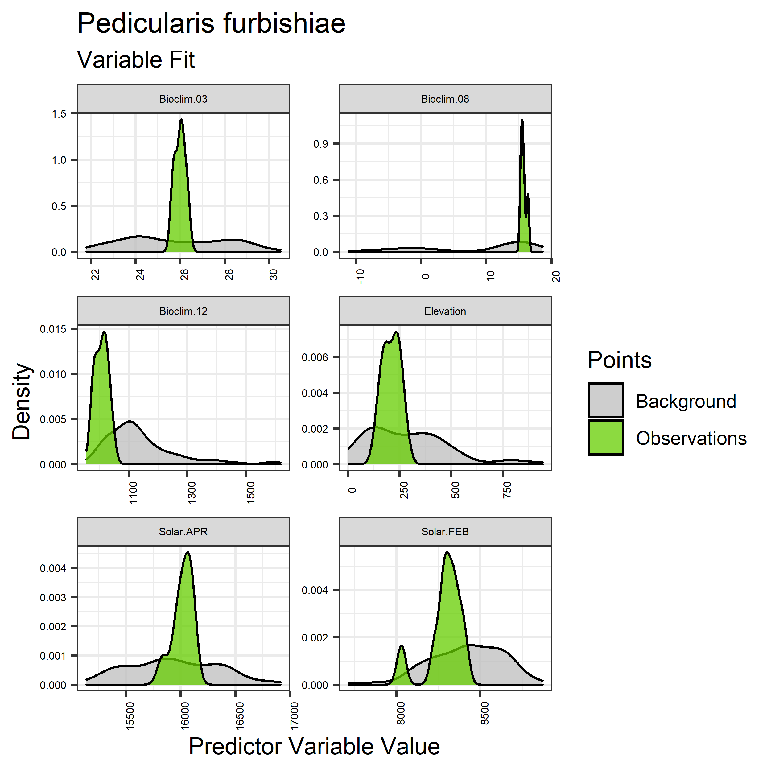
Figure 61. Sampling of continuous predictor variables retained in the best-fit Pedicularis furbishiae distribution models. Distribution of each variable at points of species occurrence (green) are contrasted with points sampled across the full modeled extent (gray).
|
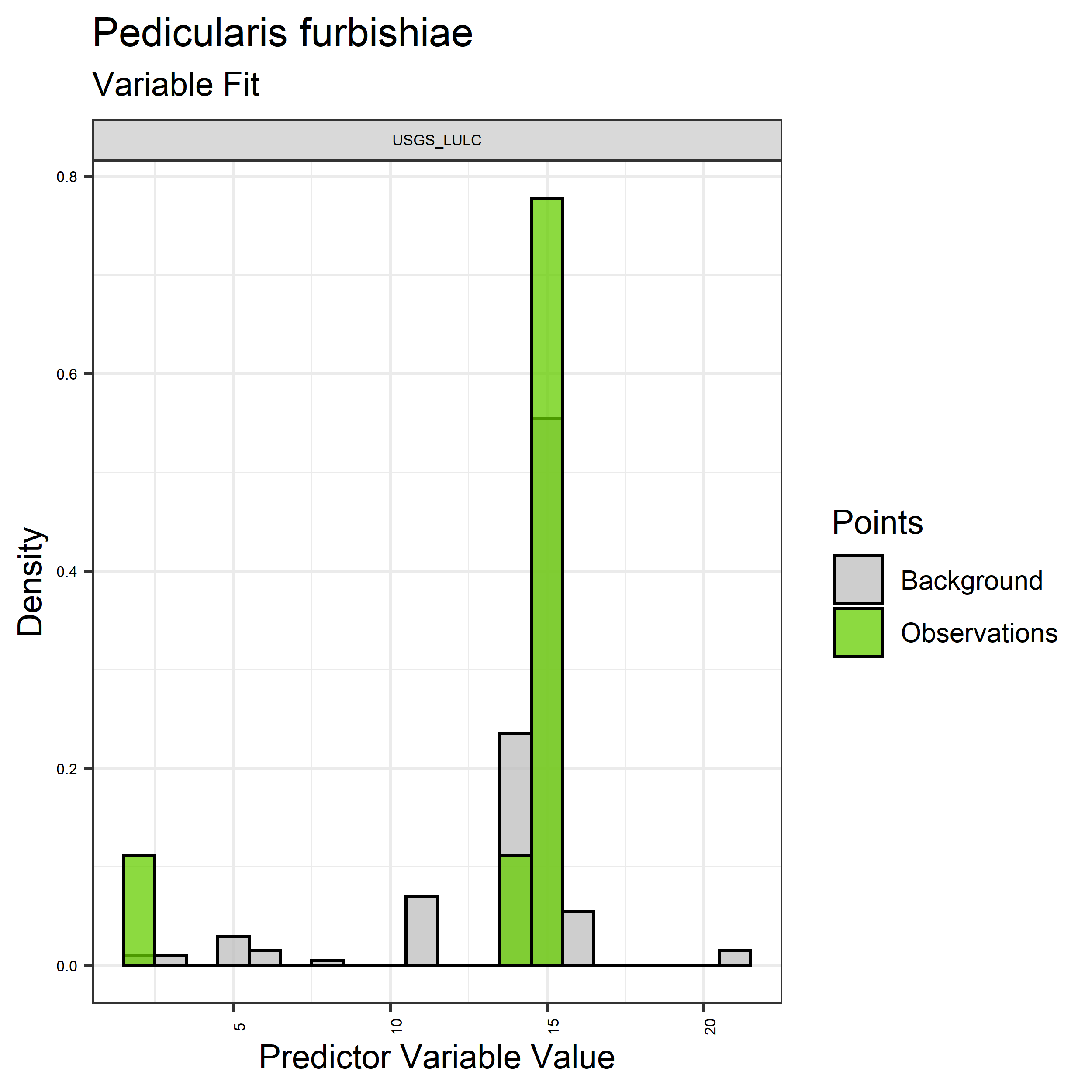
Figure 62. Sampling of discrete predictor variables retained in the best-fit Pedicularis furbishiae distribution models. Distribution of each variable at points of species occurrence (green) are contrasted with points sampled across the full modeled extent.
|
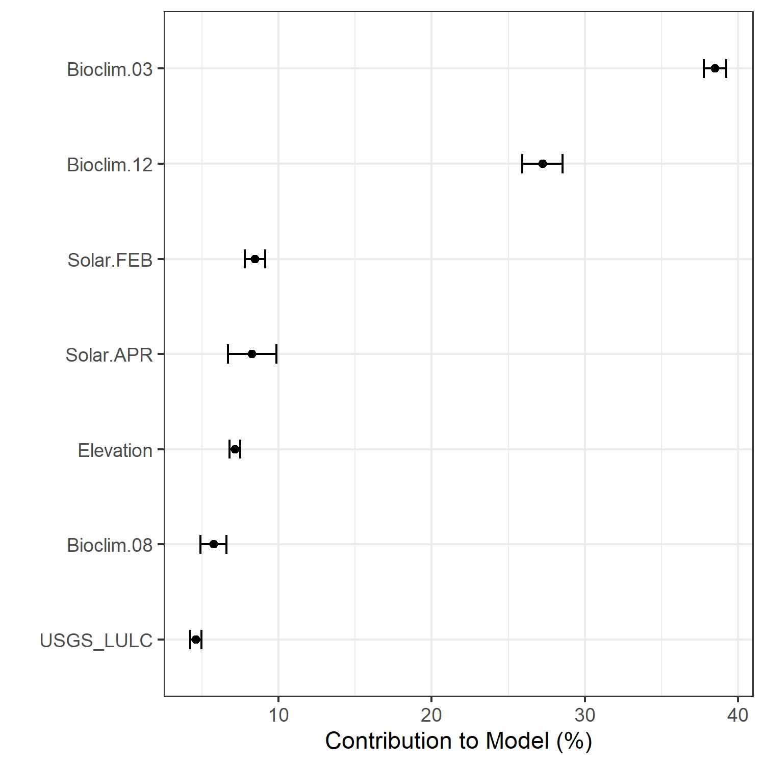
Figure 63. Percent contribution of each variable to best-fit species distribution models for Pedicularis furbishiae. Values sum to 1.0.
|
Table 30. Mean Area Under Curve (AUC) for five realizations of the best-fit SDM for Pedicularis furbishiae, calculated using 20% of species location records reserved for final evaluation.
| V1 |
V2 |
V3 |
V4 |
V5 |
mean |
sd |
| 0.996667 |
0.995556 |
0.996111 |
0.998333 |
0.996111 |
0.996556 |
0.001058 |
|
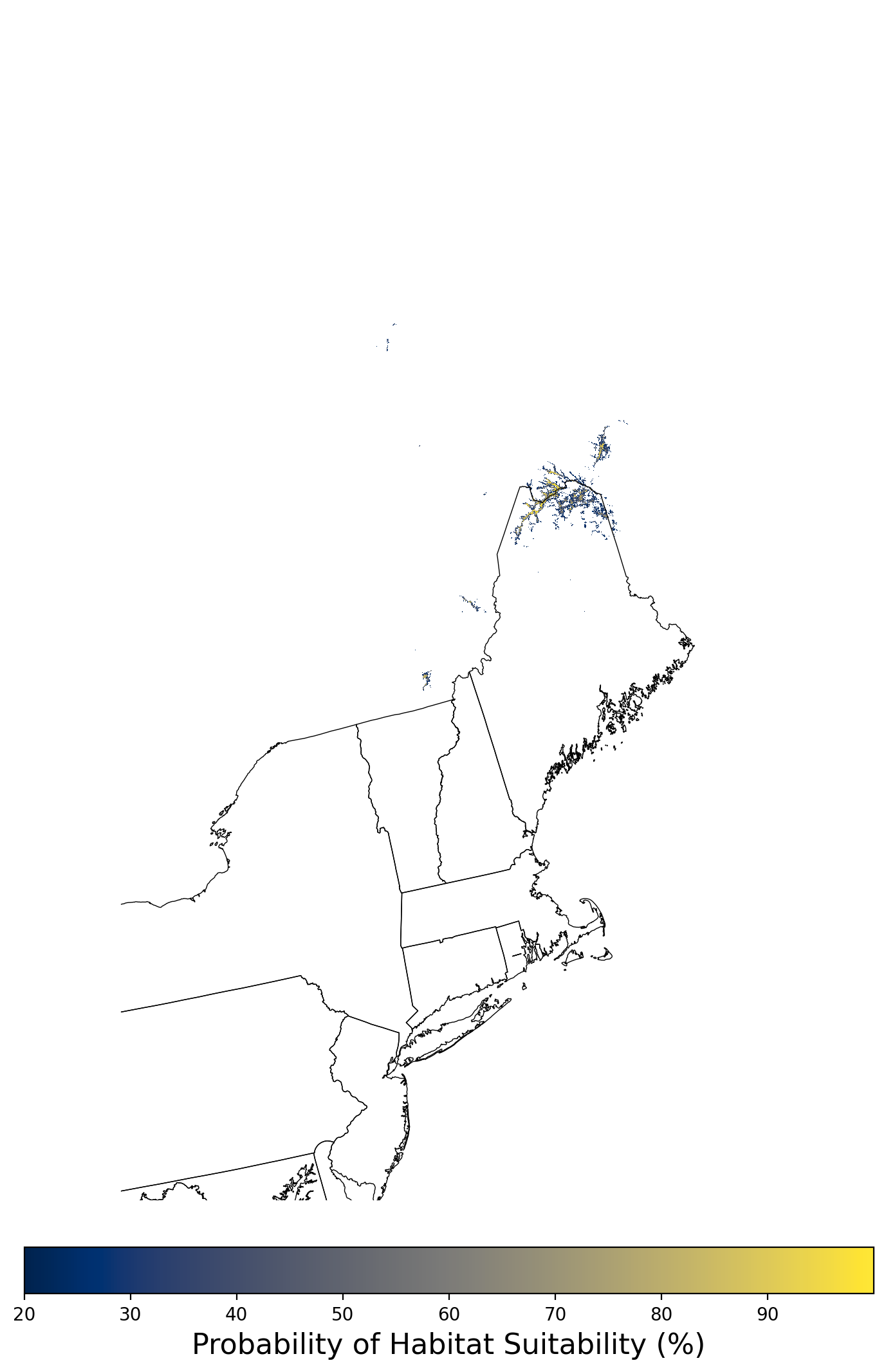
Figure 64. Final mean SDM output for Pedicularis furbishiae. |
2.2.10 Species Distribution Modeling Results for Tympanuchus cupido attwateri
The species distribution modeling results consist of the following figures and tables:
- A table showing the SDM inputs (Table 31)
- A map showing the extent of SDM coverage (Figure 65)
- A graph showing the correlation between the predictor variable selected for evaluation (Figure 66)
- A graph of the model fit of each SDM iteration as measured by total Area Under Curve (AUC) where the curve is the Receiver Operating Curve, based on training data (Figure 67)
- A table showing the diagnostic statistics of the training data used in the final selected SDM iteration (Table 32)
- Graphs illustrating the predictor variable values sampled by the species observations and randomly selected background locations for continuous variables (Figure 68), and discrete variables (Figure 69)
- A graph showing the percent contribution of each predictor variable to the final selected SDM (Figure 70)
- A table showing the mean AUC for each of the five model runs that are averaged for the final selected SDM (Table 33)
- A map of the final averaged SDM (Figure 71)
Table 31. Input parameters for species distribution modeling of Tympanuchus cupido attwateri.
| Number of predictors |
33 |
| Names of predictors |
Bioclim.01.tif, Bioclim.02.tif, Bioclim.03.tif, Bioclim.04.tif,
Bioclim.05.tif, Bioclim.06.tif, Bioclim.07.tif, Bioclim.08.tif,
Bioclim.09.tif, Bioclim.10.tif, Bioclim.11.tif, Bioclim.12.tif,
Bioclim.13.tif, Bioclim.14.tif, Bioclim.15.tif, Bioclim.16.tif,
Bioclim.17.tif, Bioclim.18.tif, Bioclim.19.tif, Elevation.tif,
Solar.APR.tif, Solar.AUG.tif, Solar.DEC.tif, Solar.FEB.tif,
Solar.JAN.tif, Solar.JUL.tif, Solar.JUN.tif, Solar.MAR.tif,
Solar.MAY.tif, Solar.NOV.tif, Solar.OCT.tif, Solar.SEP.tif,
USGS_LULC.tif |
| Predictor correlation threshold |
0.67 |
| Predictor contribution threshold |
1.0 |
| SDM threshold |
0.2 |
| Number of iterations conducted |
6 |
| Final SDM iteration number |
5 |
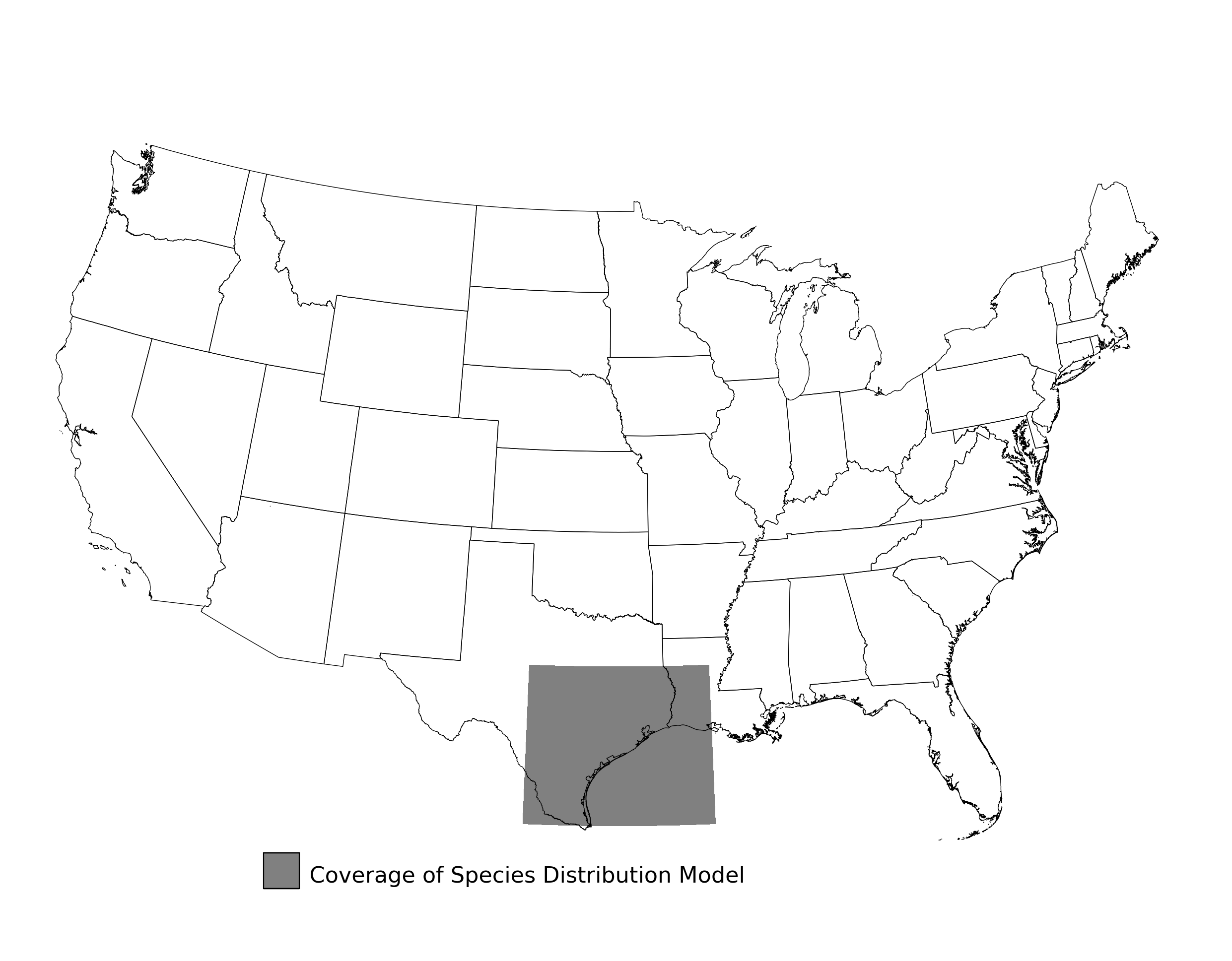
Figure 65. Extent of the species range modeled for Tympanuchus cupido attwateri. Modeling extent is determined by buffering species location records in all directions by 3 degrees latitude/longitude.
|
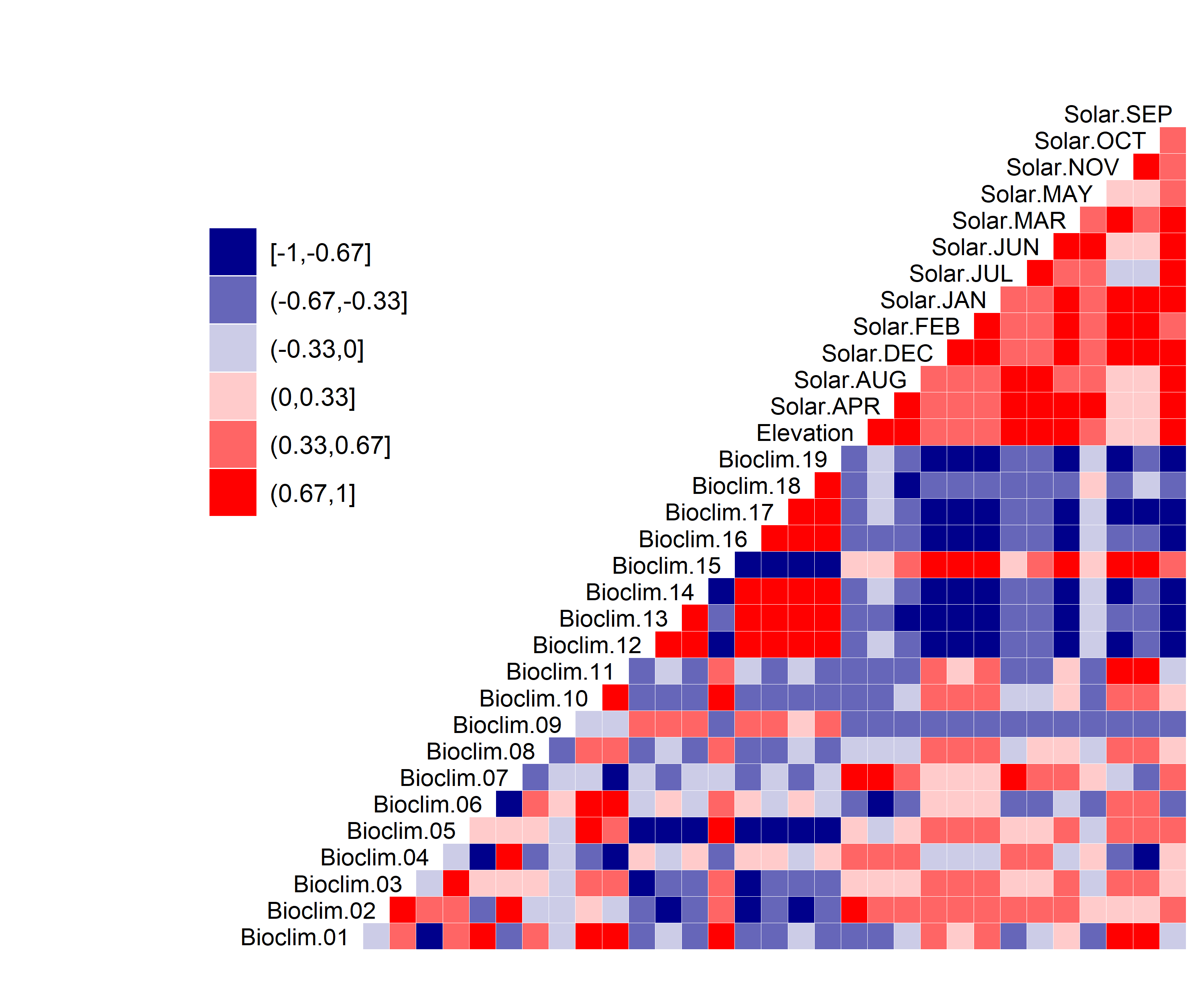
Figure 66. Correlation between SDM predictor variables for Tympanuchus cupido attwateri.
|
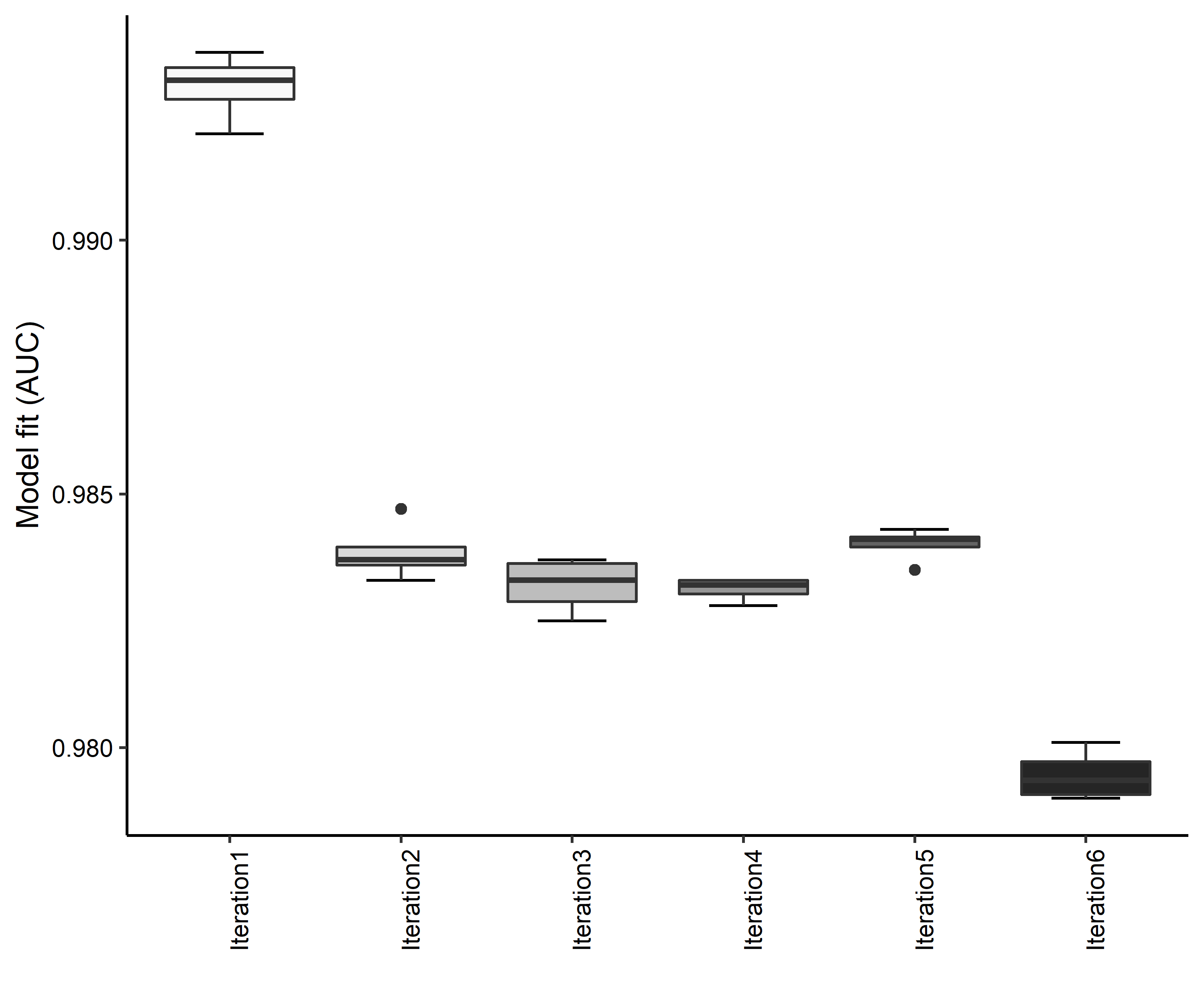
Figure 67. Boxplots of model fit for each iteration of Tympanuchus cupido attwateri distribution modeling. Statistics are calculated using 80% of species location records reserved for model training.
|
Table 32. Diagnostic statistics of the training data used in SDM iteration #5 for Tympanuchus cupido attwateri.
| Model Output |
Realization 1 |
Realization 2 |
Realization 3 |
Realization 4 |
Realization 5 |
Mean |
Standard Deviation |
| Number of training samples |
18.0000 |
18.0000 |
18.0000 |
18.0000 |
18.0000 |
18.00000 |
0.000000 |
| Regularized training gain |
2.4234 |
2.4055 |
2.4804 |
2.3710 |
2.4692 |
2.42990 |
0.045281 |
| Unregularized training gain |
3.0227 |
2.9741 |
3.0365 |
2.9800 |
3.0397 |
3.01060 |
0.031355 |
| Iterations |
240.0000 |
200.0000 |
280.0000 |
200.0000 |
340.0000 |
252.00000 |
59.329588 |
| Training AUC |
0.9847 |
0.9835 |
0.9841 |
0.9843 |
0.9841 |
0.98414 |
0.000434 |
| Number of background points |
10018.0000 |
10017.0000 |
10016.0000 |
10018.0000 |
10017.0000 |
10017.20000 |
0.836660 |
| Bioclim 18 contribution |
28.1712 |
25.4565 |
26.7546 |
27.3403 |
23.0314 |
26.15080 |
2.004633 |
| Solar APR contribution |
37.1342 |
40.1570 |
40.9931 |
36.9113 |
43.6438 |
39.76788 |
2.818317 |
| USGS_LULC contribution |
34.6945 |
34.3864 |
32.2523 |
35.7484 |
33.3248 |
34.08128 |
1.338456 |
| Bioclim 18 permutation importance |
7.6366 |
6.3329 |
3.4957 |
5.9680 |
2.8511 |
5.25686 |
2.013462 |
| Solar APR permutation importance |
83.8538 |
85.9677 |
91.9565 |
84.7369 |
90.6407 |
87.43112 |
3.639303 |
| USGS_LULC permutation importance |
8.5096 |
7.6994 |
4.5478 |
9.2951 |
6.5082 |
7.31202 |
1.857680 |
| Entropy |
6.7859 |
6.8043 |
6.7289 |
6.8396 |
6.7411 |
6.77996 |
0.045557 |
| Prevalence average probability of presence over background sites |
0.0507 |
0.0520 |
0.0480 |
0.0539 |
0.0485 |
0.05062 |
0.002451 |
| Fixed cumulative value 1 cumulative threshold |
1.0000 |
1.0000 |
1.0000 |
1.0000 |
1.0000 |
1.00000 |
0.000000 |
| Fixed cumulative value 1 Cloglog threshold |
0.0130 |
0.0146 |
0.0148 |
0.0139 |
0.0135 |
0.01396 |
0.000750 |
| Fixed cumulative value 1 area |
0.1952 |
0.1872 |
0.1801 |
0.1959 |
0.1858 |
0.18884 |
0.006682 |
| Fixed cumulative value 1 training omission |
0.0000 |
0.0000 |
0.0000 |
0.0000 |
0.0000 |
0.00000 |
0.000000 |
| Fixed cumulative value 5 cumulative threshold |
5.0000 |
5.0000 |
5.0000 |
5.0000 |
5.0000 |
5.00000 |
0.000000 |
| Fixed cumulative value 5 Cloglog threshold |
0.0944 |
0.1013 |
0.0995 |
0.1049 |
0.0929 |
0.09860 |
0.004948 |
| Fixed cumulative value 5 area |
0.1084 |
0.1067 |
0.1017 |
0.1089 |
0.1042 |
0.10598 |
0.003016 |
| Fixed cumulative value 5 training omission |
0.0000 |
0.0000 |
0.0000 |
0.0000 |
0.0000 |
0.00000 |
0.000000 |
| Fixed cumulative value 10 cumulative threshold |
10.0000 |
10.0000 |
10.0000 |
10.0000 |
10.0000 |
10.00000 |
0.000000 |
| Fixed cumulative value 10 Cloglog threshold |
0.1884 |
0.1957 |
0.1897 |
0.2056 |
0.1853 |
0.19294 |
0.008021 |
| Fixed cumulative value 10 area |
0.0783 |
0.0779 |
0.0739 |
0.0796 |
0.0751 |
0.07696 |
0.002370 |
| Fixed cumulative value 10 training omission |
0.0556 |
0.1111 |
0.0556 |
0.0556 |
0.1111 |
0.07780 |
0.030399 |
| Minimum training presence cumulative threshold |
8.2711 |
8.8995 |
8.0619 |
8.9391 |
8.4980 |
8.53392 |
0.384378 |
| Minimum training presence Cloglog threshold |
0.1550 |
0.1742 |
0.1551 |
0.1822 |
0.1562 |
0.16454 |
0.012795 |
| Minimum training presence area |
0.0864 |
0.0828 |
0.0824 |
0.0841 |
0.0818 |
0.08350 |
0.001828 |
| Minimum training presence training omission |
0.0000 |
0.0000 |
0.0000 |
0.0000 |
0.0000 |
0.00000 |
0.000000 |
| X10 percentile training presence cumulative threshold |
13.0607 |
9.2245 |
10.4669 |
10.9658 |
8.8979 |
10.52316 |
1.655762 |
| X10 percentile training presence Cloglog threshold |
0.2448 |
0.1802 |
0.1999 |
0.2201 |
0.1672 |
0.20244 |
0.031021 |
| X10 percentile training presence area |
0.0671 |
0.0812 |
0.0721 |
0.0759 |
0.0799 |
0.07524 |
0.005783 |
| X10 percentile training presence training omission |
0.0556 |
0.0556 |
0.0556 |
0.0556 |
0.0556 |
0.05560 |
0.000000 |
| Equal training sensitivity and specificity cumulative threshold |
13.0607 |
9.2245 |
10.4669 |
10.9658 |
8.8979 |
10.52316 |
1.655762 |
| Equal training sensitivity and specificity Cloglog threshold |
0.2448 |
0.1802 |
0.1999 |
0.2201 |
0.1672 |
0.20244 |
0.031021 |
| Equal training sensitivity and specificity area |
0.0671 |
0.0812 |
0.0721 |
0.0759 |
0.0799 |
0.07524 |
0.005783 |
| Equal training sensitivity and specificity training omission |
0.0556 |
0.0556 |
0.0556 |
0.0556 |
0.0556 |
0.05560 |
0.000000 |
| Maximum training sensitivity plus specificity cumulative threshold |
8.2711 |
8.8995 |
8.0619 |
8.9391 |
8.4980 |
8.53392 |
0.384378 |
| Maximum training sensitivity plus specificity Cloglog threshold |
0.1550 |
0.1742 |
0.1551 |
0.1822 |
0.1562 |
0.16454 |
0.012795 |
| Maximum training sensitivity plus specificity area |
0.0864 |
0.0828 |
0.0824 |
0.0841 |
0.0818 |
0.08350 |
0.001828 |
| Maximum training sensitivity plus specificity training omission |
0.0000 |
0.0000 |
0.0000 |
0.0000 |
0.0000 |
0.00000 |
0.000000 |
| Balance training omission predicted area and threshold value cumulative threshold |
2.1135 |
2.0353 |
2.0579 |
2.1423 |
2.0387 |
2.07754 |
0.047868 |
| Balance training omission predicted area and threshold value Cloglog threshold |
0.0347 |
0.0353 |
0.0327 |
0.0364 |
0.0331 |
0.03444 |
0.001539 |
| Balance training omission predicted area and threshold value area |
0.1492 |
0.1469 |
0.1410 |
0.1483 |
0.1448 |
0.14604 |
0.003270 |
| Balance training omission predicted area and threshold value training omission |
0.0000 |
0.0000 |
0.0000 |
0.0000 |
0.0000 |
0.00000 |
0.000000 |
| Equate entropy of thresholded and original distributions cumulative threshold |
7.9162 |
7.5065 |
7.8639 |
7.2233 |
7.9860 |
7.69918 |
0.324069 |
| Equate entropy of thresholded and original distributions Cloglog threshold |
0.1491 |
0.1489 |
0.1503 |
0.1470 |
0.1498 |
0.14902 |
0.001260 |
| Equate entropy of thresholded and original distributions area |
0.0883 |
0.0899 |
0.0835 |
0.0932 |
0.0845 |
0.08788 |
0.003974 |
| Equate entropy of thresholded and original distributions training omission |
0.0000 |
0.0000 |
0.0000 |
0.0000 |
0.0000 |
0.00000 |
0.000000 |
|
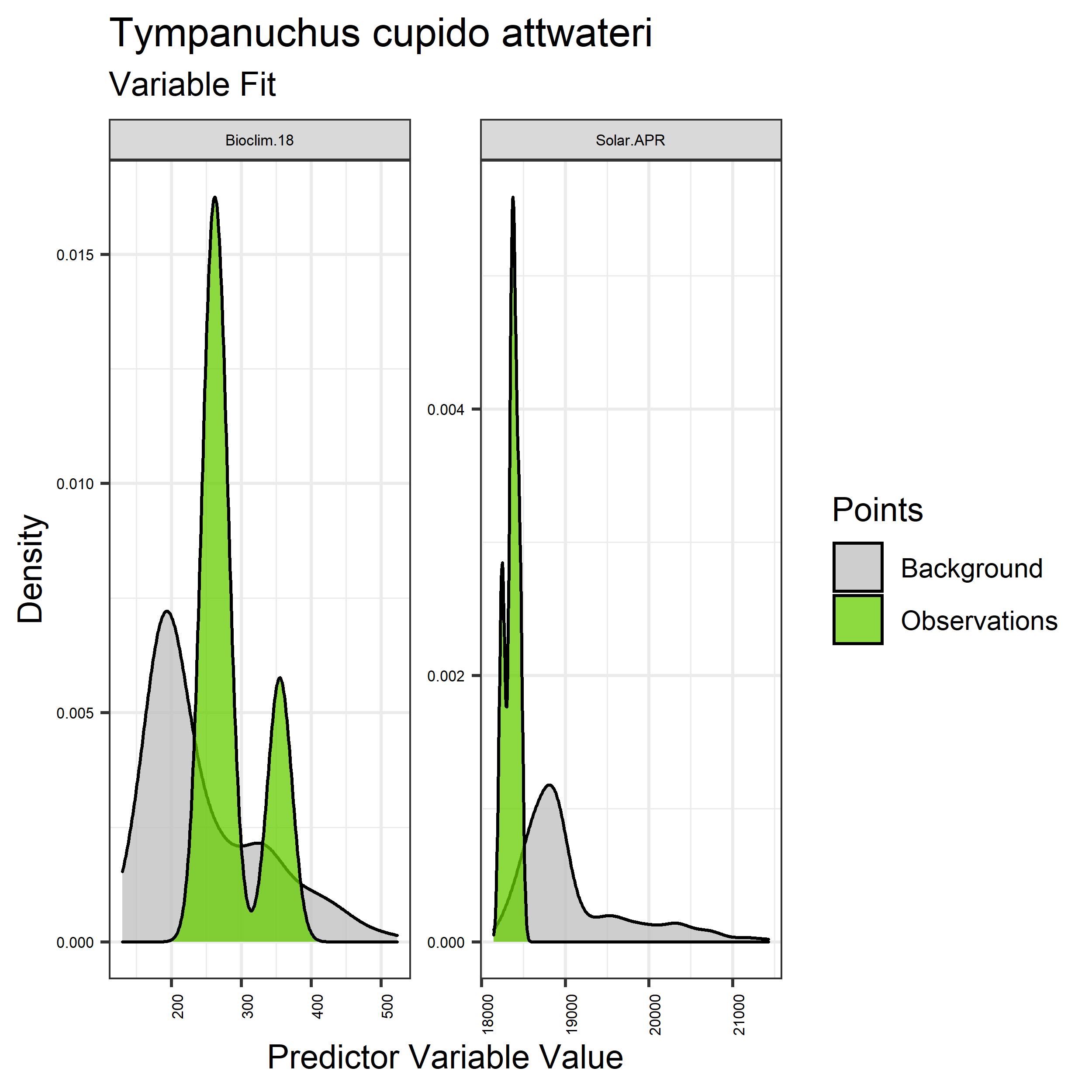
Figure 68. Sampling of continuous predictor variables retained in the best-fit Tympanuchus cupido attwateri distribution models. Distribution of each variable at points of species occurrence (green) are contrasted with points sampled across the full modeled extent (gray).
|
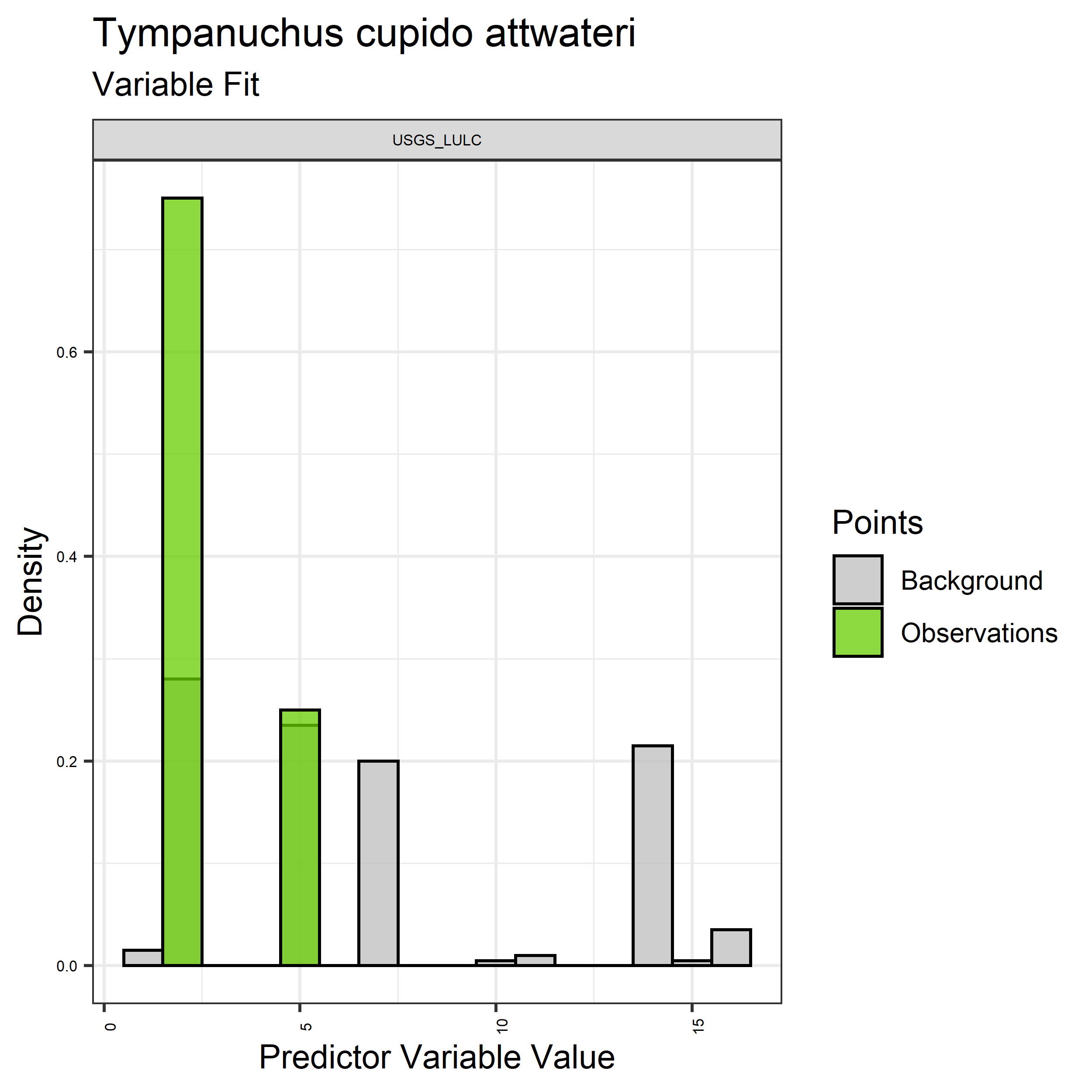
Figure 69. Sampling of discrete predictor variables retained in the best-fit Tympanuchus cupido attwateri distribution models. Distribution of each variable at points of species occurrence (green) are contrasted with points sampled across the full modeled extent.
|

Figure 70. Percent contribution of each variable to best-fit species distribution models for Tympanuchus cupido attwateri. Values sum to 1.0.
|
Table 33. Mean Area Under Curve (AUC) for five realizations of the best-fit SDM for Tympanuchus cupido attwateri, calculated using 20% of species location records reserved for final evaluation.
| V1 |
V2 |
V3 |
V4 |
V5 |
mean |
sd |
| 0.97375 |
0.97375 |
0.975 |
0.97375 |
0.9725 |
0.97375 |
0.001021 |
|
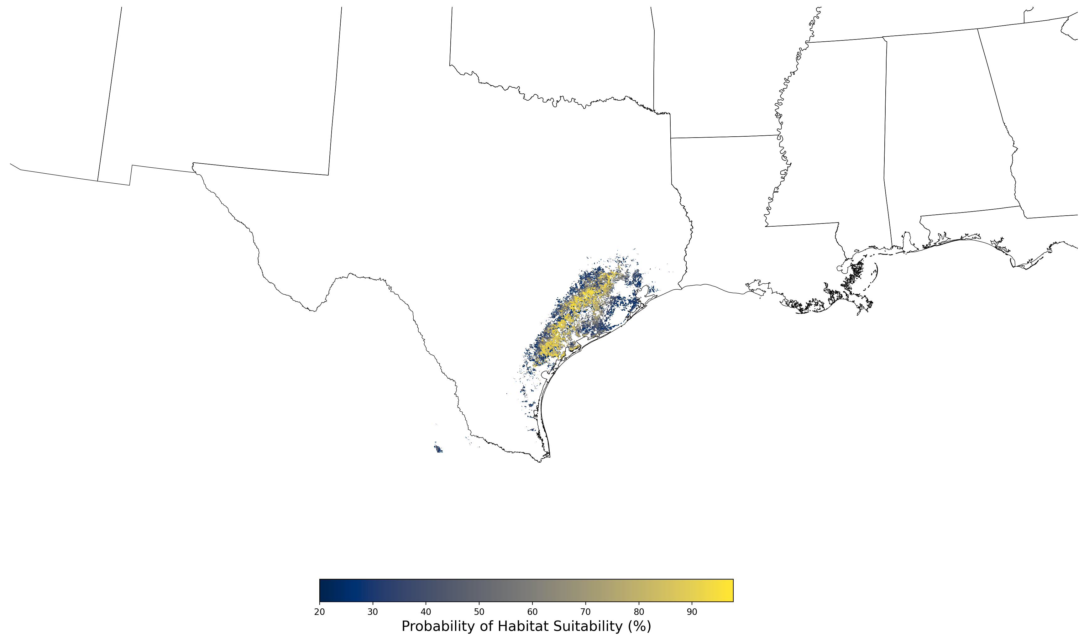
Figure 71. Final mean SDM output for Tympanuchus cupido attwateri. |
3. Co-Occurrence Modeling
3.1 Co-Occurrence Modeling Methods
APCOAT calculates probabilisic co-occurrence by multiplying probabilistic pesticide use footprints and SDM rasters. The resulting co-occurrence raster is then averaged over the entire species range and within HUC8 boundaries.
3.2 Co-Occurrence Modeling Results
- Aphelocoma coerulescens and Atrazine Applications on Corn
- Bombus affinis and Atrazine Applications on Corn
- Bufo houstonensis and Atrazine Applications on Corn
- Chamaesyce garberi and Atrazine Applications on Corn
- Cicindela puritana and Atrazine Applications on Corn
- Eurycea tonkawae and Atrazine Applications on Corn
- Lycaeides melissa samuelis and Atrazine Applications on Corn
- Neonympha mitchellii mitchellii and Atrazine Applications on Corn
- Pedicularis furbishiae and Atrazine Applications on Corn
- Tympanuchus cupido attwateri and Atrazine Applications on Corn
3.2.1 Co-Occurrence Modeling Results for Aphelocoma coerulescens and Atrazine Applications on Corn
The co-occurrence modeling results consist of the following table and figure:
- A table showing the minimum and maximum co-occurrence values calculated within HUC8 boundaries, and the average co-occurrence value for the entire species range (Table 34)
- A map of the average co-occurrence values within HUC8 boundaries (Figure 72)
Table 34. Statistics of probabilistic co-occurrence between the range of Aphelocoma coerulescens and atrazine applications on corn.
| Average co-occurrence for species range |
2.77e-02% |
| Number of HUC8 polygons included in assessment |
69 |
| Maximum average HUC8 co-occurrence |
5.91e-01% |
| Minimum average HUC8 co-occurrence |
0.00e+00% |
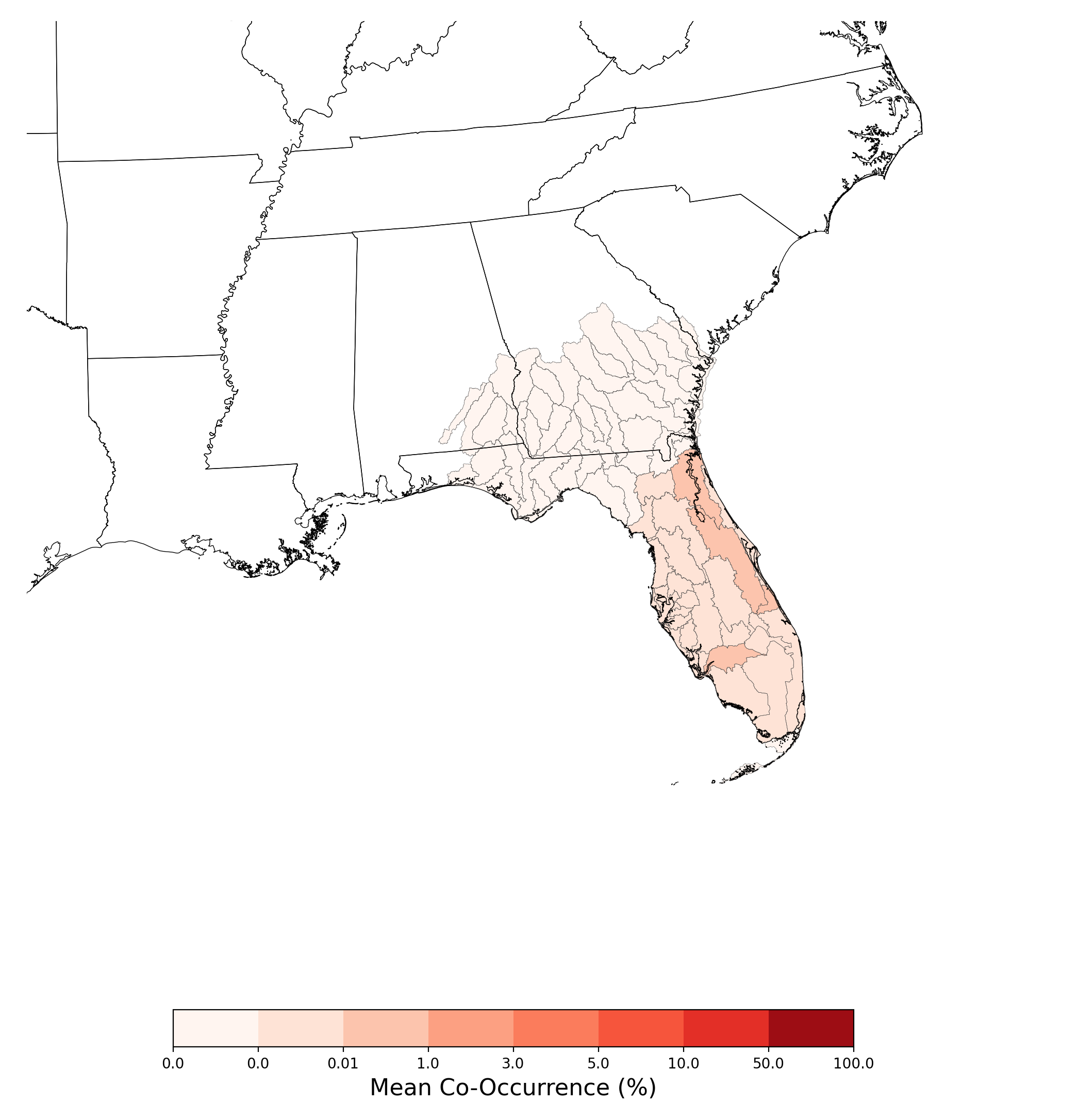
Figure 72. Map showing probabilistic co-occurrence between the range of Aphelocoma coerulescens and atrazine applications on corn, summarized at the HUC8 scale.
3.2.2 Co-Occurrence Modeling Results for Bombus affinis and Atrazine Applications on Corn
The co-occurrence modeling results consist of the following table and figure:
- A table showing the minimum and maximum co-occurrence values calculated within HUC8 boundaries, and the average co-occurrence value for the entire species range (Table 35)
- A map of the average co-occurrence values within HUC8 boundaries (Figure 73)
Table 35. Statistics of probabilistic co-occurrence between the range of Bombus affinis and atrazine applications on corn.
| Average co-occurrence for species range |
1.76e+00% |
| Number of HUC8 polygons included in assessment |
1049 |
| Maximum average HUC8 co-occurrence |
7.35e+00% |
| Minimum average HUC8 co-occurrence |
0.00e+00% |
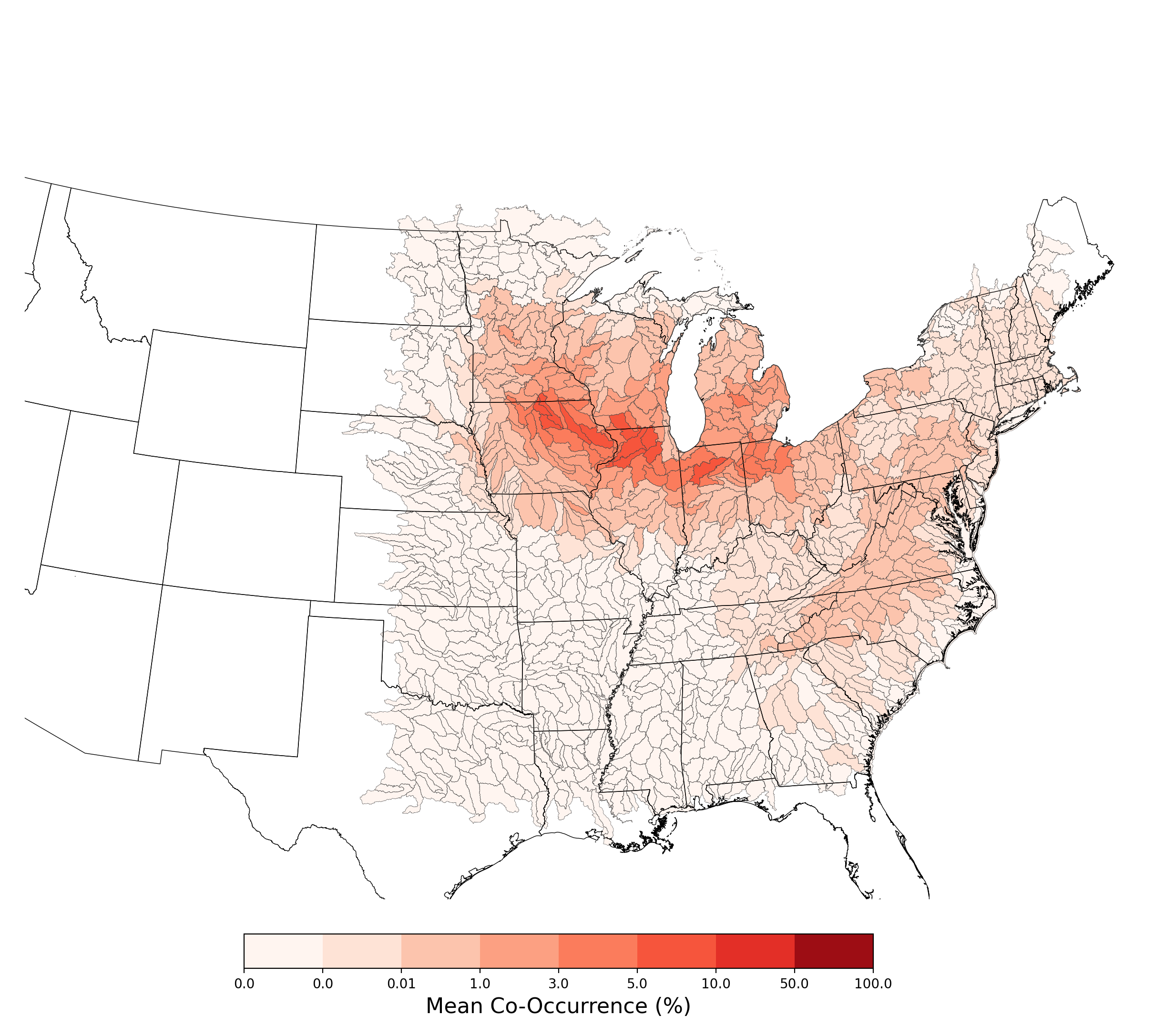
Figure 73. Map showing probabilistic co-occurrence between the range of Bombus affinis and atrazine applications on corn, summarized at the HUC8 scale.
3.2.3 Co-Occurrence Modeling Results for Bufo houstonensis and Atrazine Applications on Corn
The co-occurrence modeling results consist of the following table and figure:
- A table showing the minimum and maximum co-occurrence values calculated within HUC8 boundaries, and the average co-occurrence value for the entire species range (Table 36)
- A map of the average co-occurrence values within HUC8 boundaries (Figure 74)
Table 36. Statistics of probabilistic co-occurrence between the range of Bufo houstonensis and atrazine applications on corn.
| Average co-occurrence for species range |
4.64e-01% |
| Number of HUC8 polygons included in assessment |
162 |
| Maximum average HUC8 co-occurrence |
2.45e+00% |
| Minimum average HUC8 co-occurrence |
0.00e+00% |
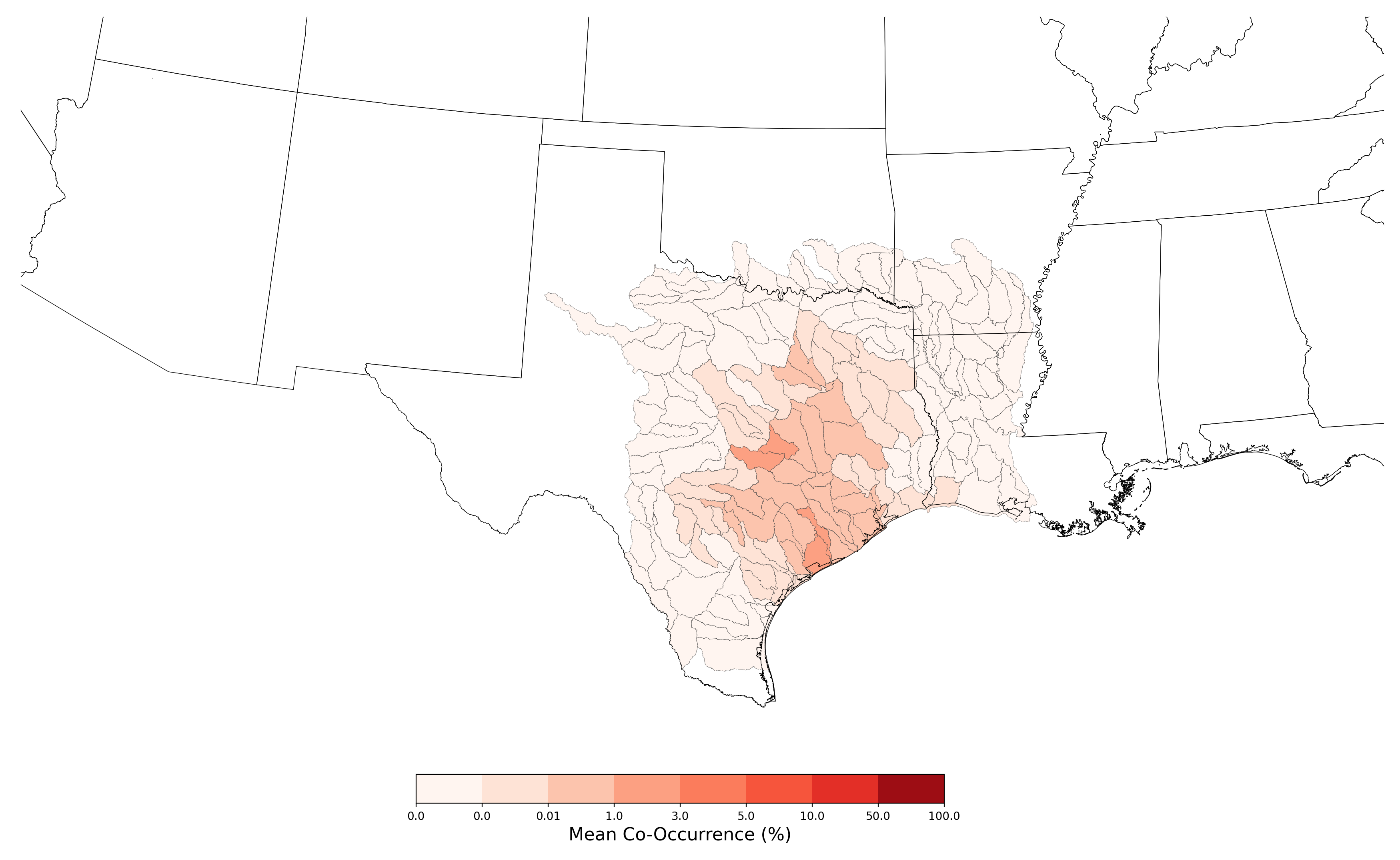
Figure 74. Map showing probabilistic co-occurrence between the range of Bufo houstonensis and atrazine applications on corn, summarized at the HUC8 scale.
3.2.4 Co-Occurrence Modeling Results for Chamaesyce garberi and Atrazine Applications on Corn
The co-occurrence modeling results consist of the following table and figure for each combination of crop and species modeled:
- A table showing the minimum and maximum co-occurrence values calculated within HUC8 boundaries, and the average co-occurrence value for the entire species range (Table 37)
- A map of the average co-occurrence values within HUC8 boundaries (Figure 75)
Table 37. Statistics of probabilistic co-occurrence between the range of Chamaesyce garberi and atrazine applications on corn.
| Average co-occurrence for species range |
3.54e-05% |
| Number of HUC8 polygons included in assessment |
22 |
| Maximum average HUC8 co-occurrence |
4.17e-05% |
| Minimum average HUC8 co-occurrence |
0.00e+00% |
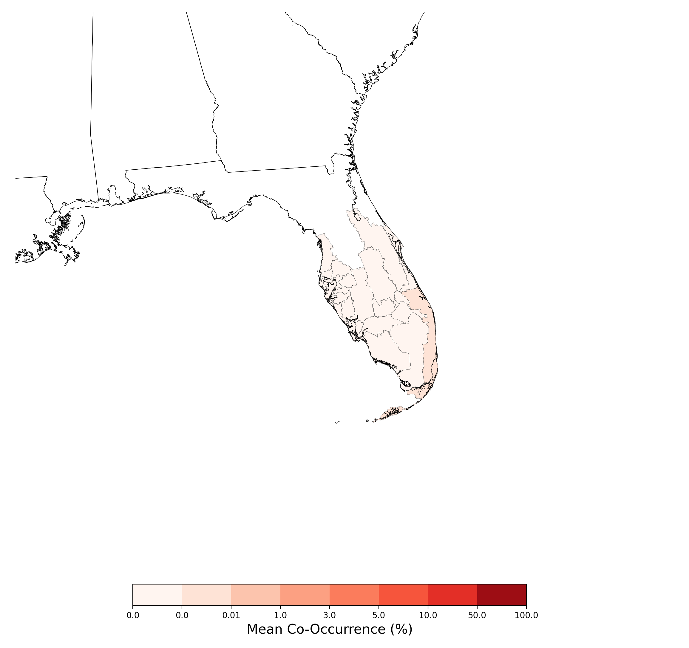
Figure 75. Map showing probabilistic co-occurrence between the range of Chamaesyce garberi and atrazine applications on corn, summarized at the HUC8 scale.
3.2.5 Co-Occurrence Modeling Results for Cicindela puritana and Atrazine Applications on Corn
The co-occurrence modeling results consist of the following table and figure for each combination of crop and species modeled:
- A table showing the minimum and maximum co-occurrence values calculated within HUC8 boundaries, and the average co-occurrence value for the entire species range (Table 38)
- A map of the average co-occurrence values within HUC8 boundaries (Figure 76)
Table 38. Statistics of probabilistic co-occurrence between the range of Cicindela puritana and atrazine applications on corn.
| Average co-occurrence for species range |
7.96e-01% |
| Number of HUC8 polygons included in assessment |
178 |
| Maximum average HUC8 co-occurrence |
2.73e+00% |
| Minimum average HUC8 co-occurrence |
0.00e+00% |
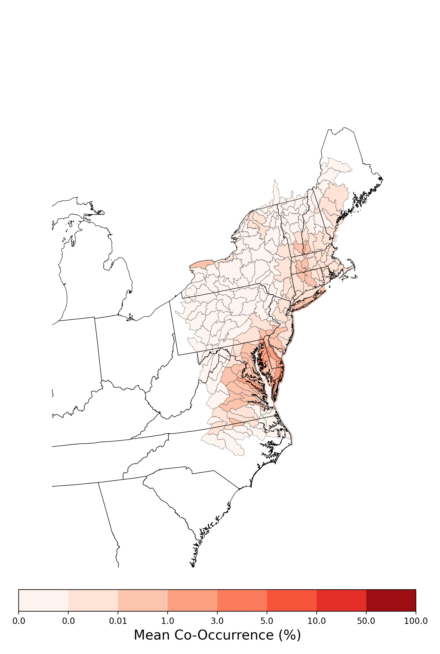
Figure 76. Map showing probabilistic co-occurrence between the range of Cicindela puritana and atrazine applications on corn, summarized at the HUC8 scale.
3.2.6 Co-Occurrence Modeling Results for Eurycea tonkawae and Atrazine Applications on Corn
The co-occurrence modeling results consist of the following table and figure for each combination of crop and species modeled:
- A table showing the minimum and maximum co-occurrence values calculated within HUC8 boundaries, and the average co-occurrence value for the entire species range (Table 39)
- A map of the average co-occurrence values within HUC8 boundaries (Figure 77)
Table 39. Statistics of probabilistic co-occurrence between the range of Eurycea tonkawae and atrazine applications on corn.
| Average co-occurrence for species range |
5.86e-03% |
| Number of HUC8 polygons included in assessment |
92 |
| Maximum average HUC8 co-occurrence |
4.74e-04% |
| Minimum average HUC8 co-occurrence |
0.00e+00% |
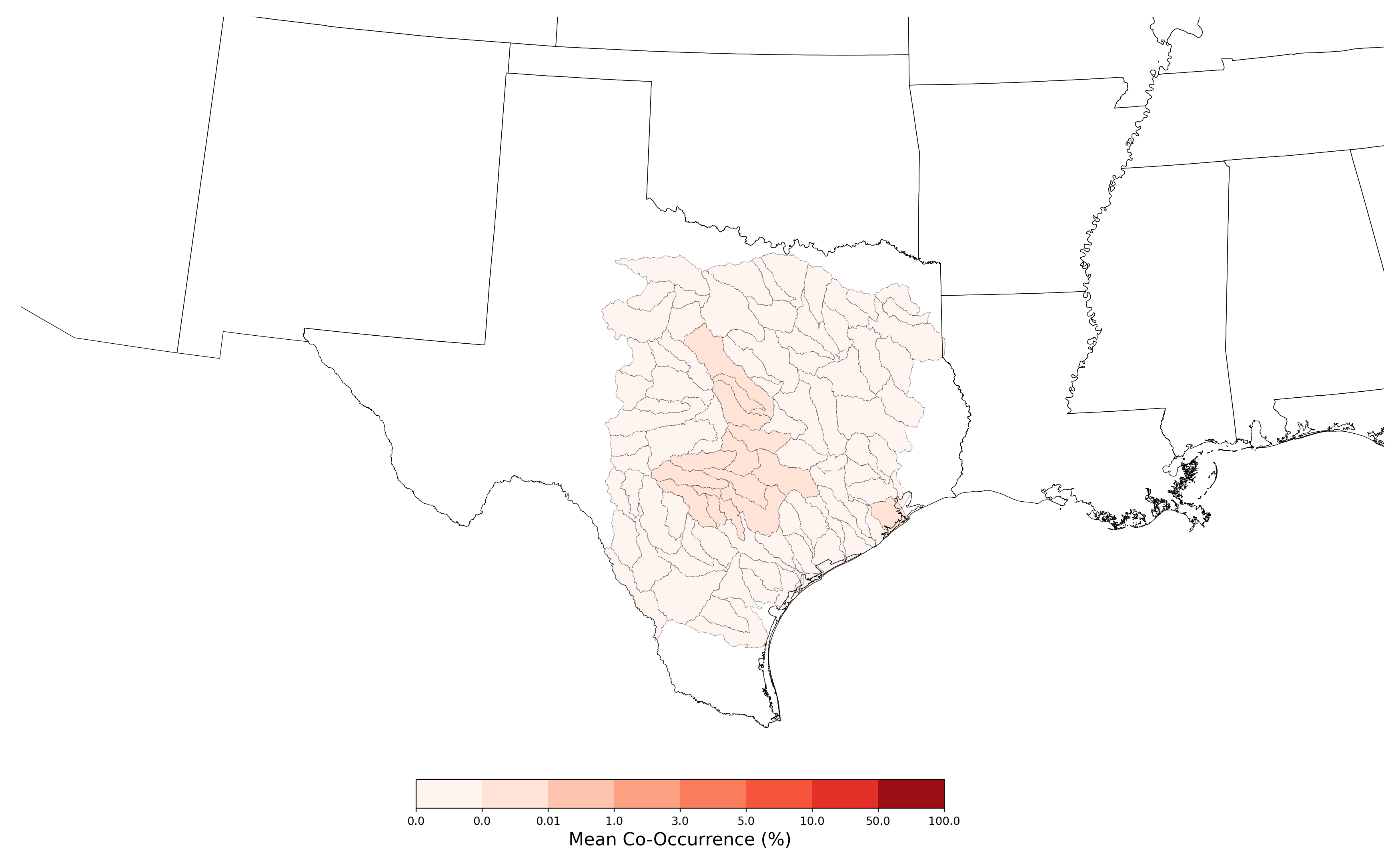
Figure 77. Map showing probabilistic co-occurrence between the range of Eurycea tonkawae and atrazine applications on corn, summarized at the HUC8 scale.
3.2.7 Co-Occurrence Modeling Results for Lycaeides melissa samuelis and Atrazine Applications on Corn
The co-occurrence modeling results consist of the following table and figure for each combination of crop and species modeled:
- A table showing the minimum and maximum co-occurrence values calculated within HUC8 boundaries, and the average co-occurrence value for the entire species range (Table 40)
- A map of the average co-occurrence values within HUC8 boundaries (Figure 78)
Table 40. Statistics of probabilistic co-occurrence between the range of Lycaeides melissa samuelis and atrazine applications on corn.
| Average co-occurrence for species range |
1.15e+00% |
| Number of HUC8 polygons included in assessment |
536 |
| Maximum average HUC8 co-occurrence |
2.51e+00% |
| Minimum average HUC8 co-occurrence |
0.00e+00% |
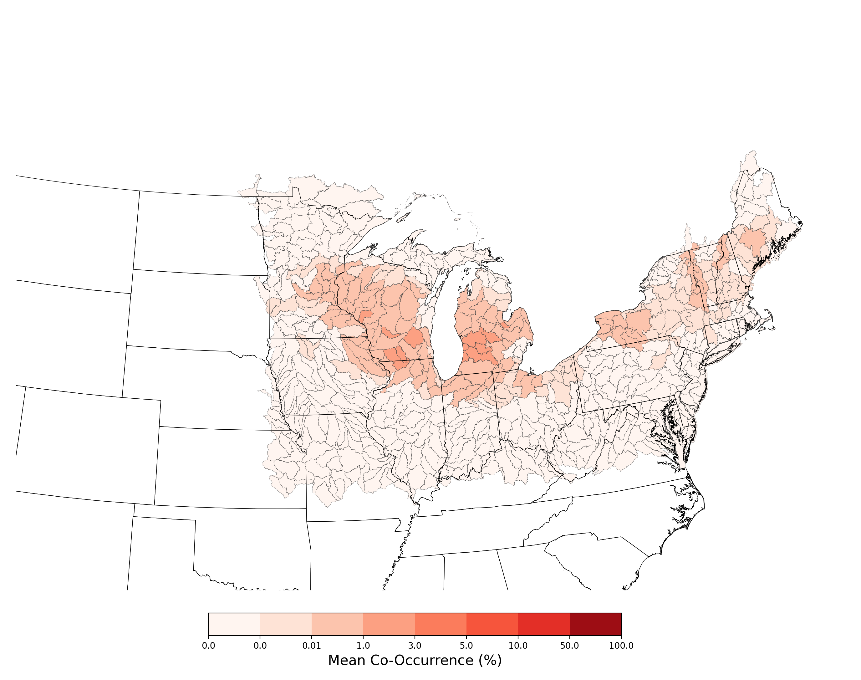
Figure 78. Map showing probabilistic co-occurrence between the range of Lycaeides melissa samuelis and atrazine applications on corn, summarized at the HUC8 scale.
3.2.8 Co-Occurrence Modeling Results for Neonympha mitchellii mitchellii and Atrazine Applications on Corn
The co-occurrence modeling results consist of the following table and figure for each combination of crop and species modeled:
- A table showing the minimum and maximum co-occurrence values calculated within HUC8 boundaries, and the average co-occurrence value for the entire species range (Table 41)
- A map of the average co-occurrence values within HUC8 boundaries (Figure 79)
Table 41. Statistics of probabilistic co-occurrence between the range of Neonympha mitchellii mitchellii and atrazine applications on corn.
| Average co-occurrence for species range |
1.51e+00% |
| Number of HUC8 polygons included in assessment |
645 |
| Maximum average HUC8 co-occurrence |
8.24e+00% |
| Minimum average HUC8 co-occurrence |
0.00e+00% |
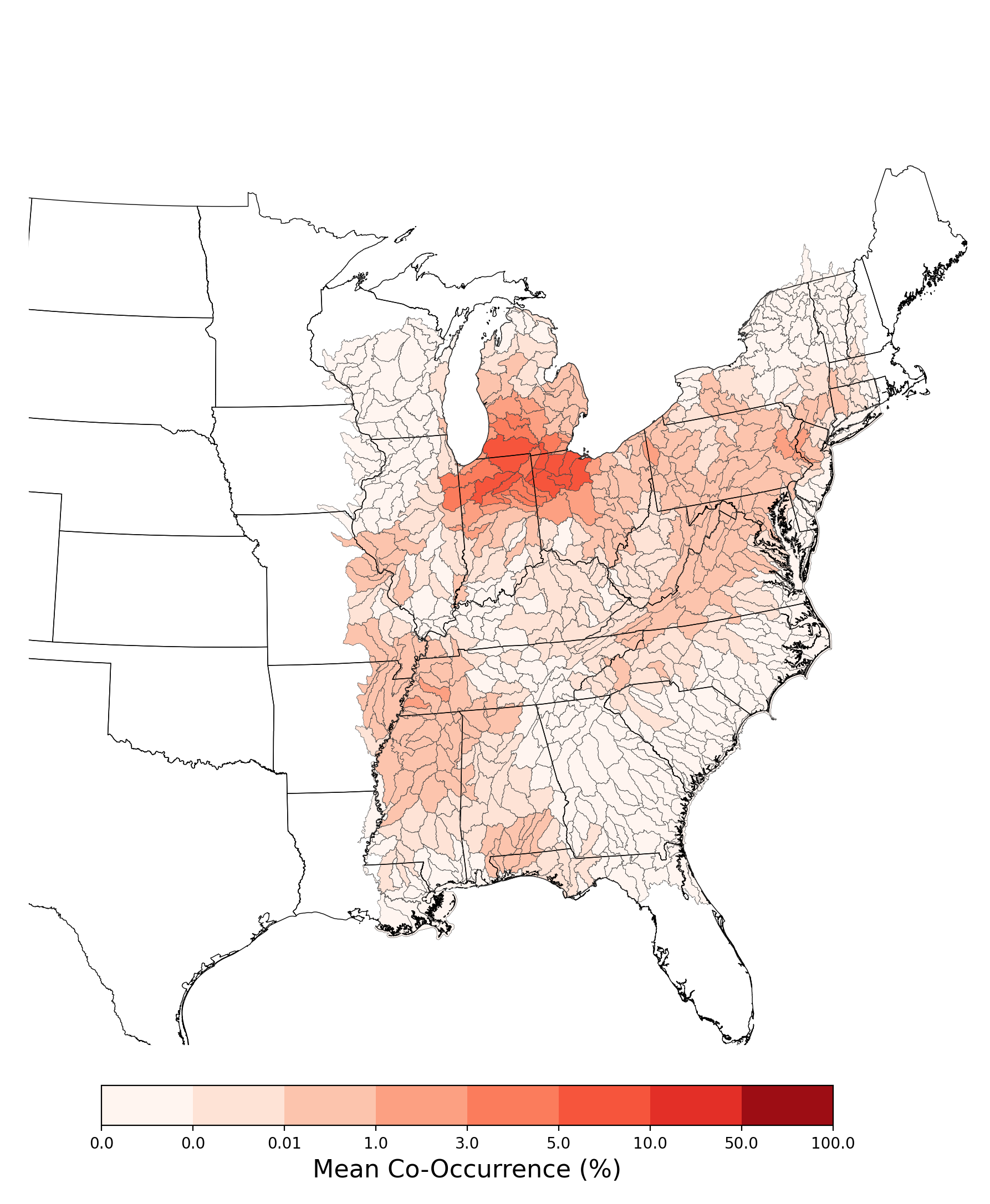
Figure 79. Map showing probabilistic co-occurrence between the range of Neonympha mitchellii mitchellii and atrazine applications on corn, summarized at the HUC8 scale.
3.2.9 Co-Occurrence Modeling Results for Pedicularis furbishiae and Atrazine Applications on Corn
The co-occurrence modeling results consist of the following table and figure for each combination of crop and species modeled:
- A table showing the minimum and maximum co-occurrence values calculated within HUC8 boundaries, and the average co-occurrence value for the entire species range (Table 42)
- A map of the average co-occurrence values within HUC8 boundaries (Figure 80)
Table 42. Statistics of probabilistic co-occurrence between the range of Pedicularis furbishiae and atrazine applications on corn.
| Average co-occurrence for species range |
7.05e-04% |
| Number of HUC8 polygons included in assessment |
32 |
| Maximum average HUC8 co-occurrence |
5.14e-04% |
| Minimum average HUC8 co-occurrence |
0.00e+00% |
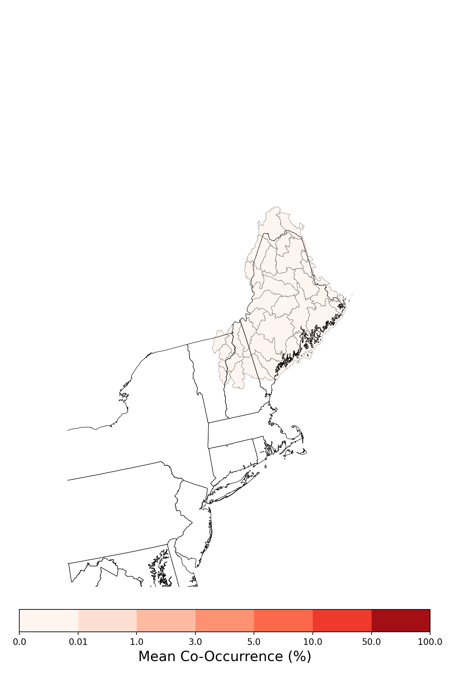
Figure 80. Map showing probabilistic co-occurrence between the range of Pedicularis furbishiae and atrazine applications on corn, summarized at the HUC8 scale.
3.2.10 Co-Occurrence Modeling Results for Tympanuchus cupido attwateri and Atrazine Applications on Corn
The co-occurrence modeling results consist of the following table and figure for each combination of crop and species modeled:
- A table showing the minimum and maximum co-occurrence values calculated within HUC8 boundaries, and the average co-occurrence value for the entire species range (Table 43)
- A map of the average co-occurrence values within HUC8 boundaries (Figure 81)
Table 43. Statistics of probabilistic co-occurrence between the range of Tympanuchus cupido attwateri and atrazine applications on corn.
| Average co-occurrence for species range |
6.72e-01% |
| Number of HUC8 polygons included in assessment |
112 |
| Maximum average HUC8 co-occurrence |
1.61e+00% |
| Minimum average HUC8 co-occurrence |
0.00e+00% |
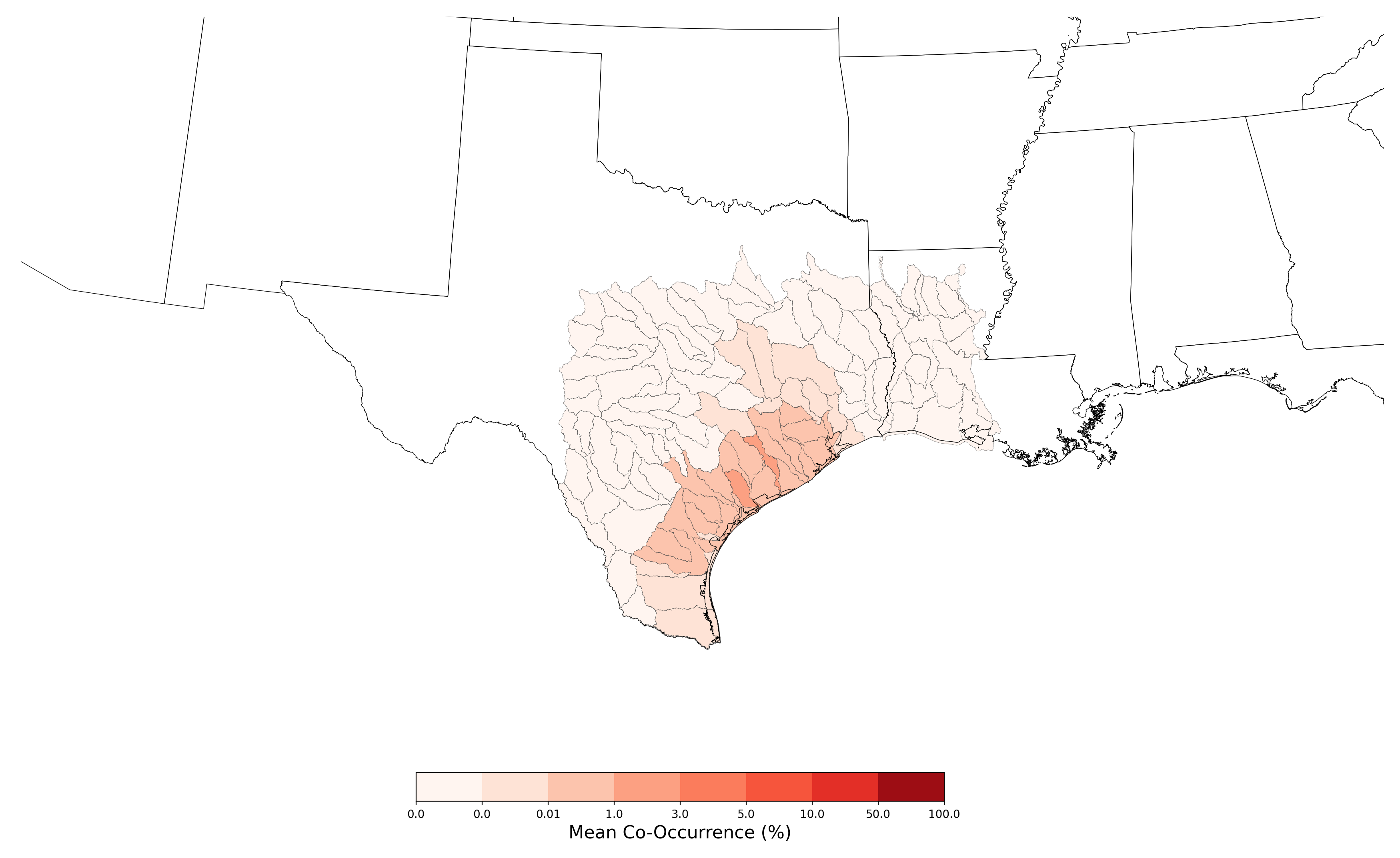
Figure 81. Map showing probabilistic co-occurrence between the range of Tympanuchus cupido attwateri and atrazine applications on corn, summarized at the HUC8 scale.
4. Summary
In this assessment probabilistic spatial co-occurrence was calculated for applications of atrazine on corn and the distributions of 10 endangered species. The probability that corn was planted in a given location was calculated using six years of remotely sensed crop maps[6] and crop production surveys[8], and the probability that those locations were treated with atrazine was calculated using six years of estimates of atrazine usage[3]. The probability that a given location provided suitable habitat for the species of interest was calculated using maximum entropy methods to identify areas where environmental conditions (Table 44) were similar to the conditions at locations where the species have been observed. Environmental conditions were modeled using solar radiation, bioclimatic, and elevation datasets[10], and land use/land cover data[11]. Species location data were provided by NatureServe[13].
Table 44. Environmental variables used to predict species habitat suitability, ranked by importance.
| Species |
Environmental Variable - Importance |
Average Species Spatial Co-Occurrence with Atrazine Applications |
Florida scrub jay
(Aphelocoma coerulescens) |
- Temperature Seasonality (standard deviation x100) - 56.1%
- Mean Temperature of Driest Quarter - 10.0%
- Precipitation of Warmest Quarter - 9.6%
- Solar Radiation, August - 9.3%
- Solar Radiation, May - 7.7%
- Elevation - 5.5%
- Land Use/Land Cover - 1.7%
|
2.77e-02% |
Rusty patched bumble bee
(Bombus affinis) |
- Solar Radiation, September - 67.6%
- Land Use/Land Cover - 10.3%
- Precipitation of Driest Quarter - 9.5%
- Mean Diurnal Range (Mean of monthly (max temp - min temp)) - 7.3%
- Elevation - 5.3%
|
1.76e+00% |
Houston toad
(Bufo houstonensis) |
- Precipitation of Driest Quarter - 56.7%
- Mean Temperature of Coldest Quarter - 36.1%
- Land Use/Land Cover - 7.1%
|
4.64e-01% |
Garber's spurge
(Chamaesyce garberi) |
- Mean Diurnal Range (Mean of monthly (max temp - min temp)) - 44.8%
- Isothermality (Mean Diurnal Range/Temperature Annual Range) - 31.4%
- Solar Radiation, June - 15.7%
- Precipitation Seasonality (Coefficient of Variation) - 4.1%
- Precipitation of Wettest Month - 0.3%
|
3.54e-05% |
Puritan tiger beetle
(Cicindela puritana) |
- Elevation - 68.6%
- Precipitation Seasonality (Coefficient of Variation) - 20.4%
- Precipitation of Wettest Month - 7.9%
- Land Use/Land Cover - 2.2%
- Solar Radiation, October - 0.8%
|
7.96e-01% |
Jollyville plateau salamander
(Eurycea tonkawae) |
- Elevation - 55.3
- Mean Diurnal Range (Mean of monthly (max temp - min temp)) - 28.6%
- Isothermality (Mean Diurnal Range/Temperature Annual Range) - 10.6%
- Temperature Seasonality (standard deviation x100) - 5.0%
- Land Use/Land Cover - 0.5%
|
5.86e-03% |
Karner blue butterfly
(Lycaeides melissa samuelis) |
- Solar Radiation, October - 43.9%
- Isothermality (Mean Diurnal Range/Temperature Annual Range) - 21.7%
- Solar Radiation, March - 14.9%
- Precipitation of Wettest Month - 12.7%
- Precipitation Seasonality (Coefficient of Variation) - 4.5%
- Mean Temperature of Wettest Quarter - 2.3%
|
1.15e+00% |
Mithcell's satyr
(Neonympha mitchellii mitchellii) |
- Solar Radiation, September - 28.1%
- Mean Temperature of Wettest Quarter - 22.9%
- Elevation - 16.5%
- Temperature Annual Range - 10.2%
- Mean Diurnal Range (Mean of monthly (max temp - min temp)) - 9.1%
- Land Use/Land Cover - 7.5%
- Precipitation of Driest Month - 5.7%
|
1.51e+00% |
Furbish's lousewort
(Pedicularis furbishiae) |
- Annual Precipitation - 33.5%
- Isothermality (Mean Diurnal Range/Temperature Annual Range) - 29.1%
- Elevation - 19.6%
- Solar Radiation, April - 10.1%
- Solar Radiation, February - 4.1%
- Mean Temperature of Wettest Quarter - 3.3%
- Land Use/Land Cover - 0.3%
|
7.05e-04% |
Attwater's prairie chicken
(Tympanuchus cupido attwateri) |
- Solar Radiation, April - 87.4%
- Land Use/Land Cover - 7.3%
- Precipitation of Warmest Quarter - 5.3%
|
6.72e-01% |
5. References
1. Dunne, J., Richardson, L., Rathjens, H., Winchell, M. (2022). Automated Probabilistic Co-Occurrence Assessment Tool. Stone Environmental Inc., Montpelier, Vermont. https://www.stone-env.com/APCOAT
2. Budreski, K., Winchell, M., Padilla, L., Bang, J., & Brain, R. A. (2016). A probabilistic approach for estimating the spatial extent of pesticide agricultural use sites and potential co-occurrence with listed species for use in ecological risk assessments. Integrated Environmental Assessment and Management, 12(2), 315-327. https://doi.org/10.1002/ieam.1677
3. Wieben, C.M.,(2019). Estimated Annual Agricultural Pesticide Use by Major Crop or Crop Group for States of the Conterminous United States, 1992-2017 (ver. 2.0, May 2020): U.S. Geological Survey data release, https://doi.org/10.5066/P9HHG3CT
4. Phillips, S.J., Anderson, R.P., Dudík, M., Schapire, R.E., Blair, M.E. (2017). Opening the black box: an open-source release of Maxent. Ecography. 40(7):887-893. https://doi.org/10.1111/ecog.03049
5. Elith, J., Phillips, S. J., Hastie, T., Dudík, M., Chee, Y. E., & Yates, C. J. (2011). A statistical explanation of MaxEnt for ecologists. Diversity and distributions, 17(1), 43-57. https://doi.org/10.1111/j.1472-4642.2010.00725.x
6. United States Department of Agriculture, National Agricultural Statistics Service. (2019). Cropland data layer. https://nassgeodata.gmu.edu/CropScape/
7. United States Department of Agriculture, National Agricultural Statistics Service. (2020). Cropland Data Layer - Metadata. https://www.nass.usda.gov/Research_and_Science/Cropland/metadata/meta.php
8. USDA - National Agricultural Statistics Service - Census of Agriculture. (2021). https://www.nass.usda.gov/AgCensus/
9. Syngenta Crop Protection LLC. (2013). AAtrex4L: Product Label. Greensboro, North Carolina
10. Fick, S.E., Hijmans, R.J. (2017). WorldClim 2: new 1-km spatial resolution climate surfaces for global land areas. International Journal of Climatology. 37(12):4302-4315. https://doi.org/10.1002/joc.5086. Data retrieved from https://www.worldclim.org on April 2021.
11. Brown, J. F., Loveland, T. R., Merchant, J. W., Reed, B. C., & Ohlen, D. O. (1993). Using multisource data in global land-cover characterization: Concepts, requirements, and methods. Photogrammetric Engineering and Remote Sensing, 59(6), 977-987. https://pubs.er.usgs.gov/publication/70187631
12. Richardson, L., Dunne, J., Feken, M., Brain, R., Ghebremichael, L., & Winchell, M. (2021). Probabilistic co-occurrence assessment for suites of listed species. Integrated environmental assessment and management. https://doi.org/10.1002/ieam.4542
13. NatureServe. (2002). Element occurrence data standard. http://downloads.natureserve.org/conservation_tools/element_occurence_data_standard.pdf