More than 1,600 animal, plant, and other species are listed as threatened or endangered under the Endangered Species Act (ESA) by the US Fish and Wildlife Service (USFWS), whose mission is to prevent the extinction of these sensitive species and take actions to allow population recovery and eventual delisting. Under Section 7 of the Act, federal agencies are required to consult with USFWS and the National Marine Fisheries Service (NMFS) to evaluate whether their actions may affect listed species protected by the ESA[12]. For example, the US Environmental Protection Agency (EPA) regulates the sale of more than 1,000 pesticide chemicals, each of which is required by law to go through this consultation process, in which the USFWS and/or NMFS must issue a Biological Opinion regarding potential risks to listed species. Despite this legal requirement, few pesticides have undergone the consultation process, perhaps due to interagency disagreements about interpretation of the law or poorly defined methods. A 2013 National Research Council[13] study described a method for conducting these consultations, known as Biological Evaluations (BE), in which a preliminary determination for each listed species is made, in part, based on the degree of spatial overlap between pesticide usage areas and the species' range or Critical Habitat maps. Following publication of this study, USFWS conducted several preliminary consultations on pesticides regulated by EPA[14, 15, 16], later clarifying that >1% spatial concurrence between pesticide usage areas and listed species habitats was a threshold for a 'may affect' determination[14]. In the event of such a 'may affect' decision, BEs use a weight-of-evidence approach to evaluate exposure and toxicity data in consultation with USFWS.
The current BE model has not been effective for regulatory agencies or industry and may not be appropriately assessing potential risks to listed species. The method is deterministic (i.e., presence/absence), identifying simple spatial overlap between listed species ranges and crop footprints. The species range datasets are often poorly modeled or of low spatial resolution, and the crop footprints do not reflect variable patterns of crop production or pesticide usage. Such methods may either under- or over-predict pesticide exposure risk, benefiting neither listed species nor the parties involved. In recent work, a team of scientists at Syngenta Crop Protection and Stone Environmental has addressed some of these challenges by developing probabilistic models of pesticide use patterns and species distributions[1, 2, 18, 19]. To address the high number of species protected by the ESA and pesticide products regulated by EPA, in ongoing research in 2019-2020 we apply these methods to suites of listed species co-occurring in delimited geographic areas (i.e., watersheds). USFWS recently published standard operating procedures for characterizing listed species distributions that are expected to improve the rigor of co-occurrence analysis, and follow similar methods to those used in our own work.
The scope and aim of this software is to provide users with the ability to rapidly implement the methods we have developed to assess probabilistic co-occurrence between pesticide use and species of interest for the purposes of regulatory review. With APCOAT, users are able to use pesticide application rates and species locations to generate automated reports detailing pesticide usage, species distribution modeling, and co-occurrence between the two (Figure 1). This guide walks users through each APCOAT function in a step-by-step manner and includes descriptions of the methods and processing involved in each model. These methods have been peer-reviewed and published in several research manuscripts, and more detailed descriptions of the models are cited in the References section.
APCOAT will run on most 64-bit Windows 10 machines. However, generating use footprints, species distribution models, and co-occurrence summaries may require several hours of processing time. We recommend
beginning co-occurrence assessments using a subset of species of interest to determine the general rate of processing time before completing large batches of species assessments.
Example processing times for an analysis of one pesticide applied to two crops, two SDMs, and the four resulting co-occurrence reports:
Running APCOAT to generate co-occurrence reports consists of four separate processes:
5.1 Project Management to create, save, and load the project database and associated folders
5.2 Pesticide Use Footprints to generate probabilistic maps of the likelihood of crop cultivation at 30 m² resolution, and that the given crop will be treated with a pesticide of interest
5.3 Species Distribution Modeling to generate probabilistic maps of habitat quality for a given species
5.4 Co-Occurrence Assessment to multiply the pesticide use footprints and species distribution models and produce a co-occurrence raster and report summarizing modeling methods, inputs, and outputs
|
Methods
APCOAT projects consists of a project folder paired with a project database. Renaming, editing, or moving any files created by APCOAT in this folder will corrupt database connections. To further process or analyze outputs created by APCOAT, create a copy of the data in a new folder. Associated project sub-folders paired with project databases are used to store the raster and statistical outputs for each process.
To create a project database and associated output sub-folders:
- - Click the "File" menu on the upper left corner of the window.
- - Select "New".
- - Select an empty destination folder.
- - Provide a project file name. APCOAT will generate the following files and be named as shown below:
- A project database used to store user inputs
- A folder used to store results of co-occurrence analyses
- A folder used to store results of species distribution modeling
- A folder used to store results of pesticide usage modeling
- - Project progress may be saved at any time that APCOAT is not actively processing data. The file menu is also used to load previously saved projects.
|

|
|
Methods
APCOAT pesticide use footprints are generated by multiplying probabilistic crop footprints by estimates of the Percent Crop Treated (PCT) (Figure 1). The method for producing the probabilistic crop footprints incorporates best available information at the time of analysis from the Cropland Data Layer (CDL)[21] for 6 years (2016 - 2021).
The PCT rasters are created by first calculating a time series of the maximum potential annual usage in a region. Maximum annual usage is calculated by multiplying the regional crop acreage measured from CDL for 6 years by the specified application rates. Regional pesticide usage data is then divided by the maximum potential usage in each year to generate a time series of annual PCT calculations for each region. Finally, a user-specified statistic is calculated from these regional time series and converted to raster format. The PCT rasters are then multiplied by probabilistic crop footprint rasters.
Offsite transport for processes such as pesticide drift and runoff may also be modeled at user-specified distances. With this feature, pesticide usage probabilities are extended in rings around usage sites, with the usage probability being evenly distributed around the ring. For example, a single 30m usage footprint pixel with a usage probability of 50% is surrounded by 8 pixels, so a 30m transport distance applied to this footprint will also show a 6.25% pesticide presence probability in each of the surrounding pixels (50% / 8 = 6.25%),
|

|
To create probabilistic pesticide use footprints:
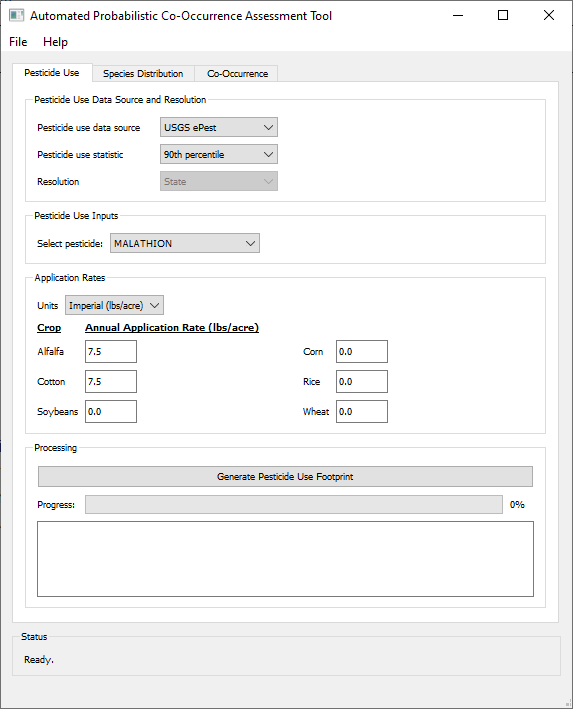
- - Click the "Pesticide Use" tab.
- - Select one of the following the pesticide use data sources. Note that your selection will modify the appearance of the subsequent input fields and may not match the example screenshot:
- - USGS ePest: Usage estimates compiled by USGS for years 2012 - 2019[3]
- USGS ePest High - unreported use in CRD surveys is assumed to be missing data, and is estimated using neighboring or regional CRDs
- USGS ePest Low - unreported use is assumed to be accurate
- USGS ePest Combined - compiled estimates from ePest High and ePest low
- - Custom Usage (USGS Groups): Usage data provided by the user. See below for Preparing Custom Usage Data
- - Custom Usage (User-defined Groups): Usage data provided by the user. See below for Preparing Custom Usage Data
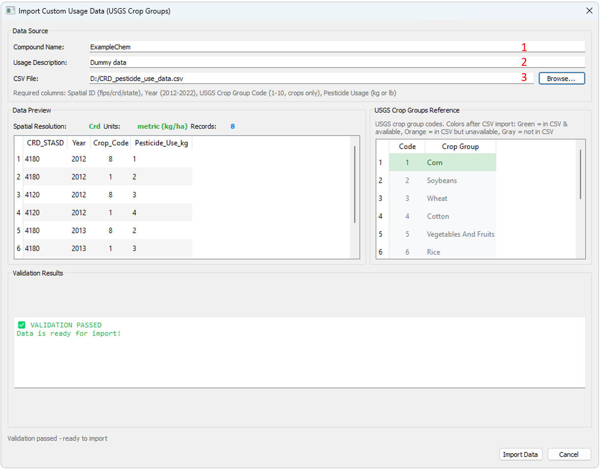
- Enter the compound name
- Enter a short description of the usage data source
- Navigate to the custom usage data source. For USGS Groups, ensure that the "Crop_Code" field values conform to the codes listed below. For User-defined Groups, ensure that the "Crop_Group" field values are non-numerical and consistent across years and regions.
- - 100% Crop Treated: No usage data is used and all usage sites are assumed to be treated
- - Select the desired pesticide use statistic. This will be calculated for each region of interest over the specified annual time series.
- - Select the desired spatial resolution, which is dependent on the pesticide use data source.
- - USGS ePest estimates are published by state, the only available spatial resolution will be "State" if it is selected as the pesticide use data source.
- - Custom (CSV file) data may be provided at the county, Crop Reporting District, or state scale, and the resolution will be automatically detected from the file header. If you wish to summarize the data you have provided at a larger spatial scale, select that scale from the Resolution options.
- - Select or name the pesticide of interest, depending on pesticide use data source:
- - USGS ePest select one of the 315 pesticides available from the ePest database.
- - Custom select the name of the imported pesticide
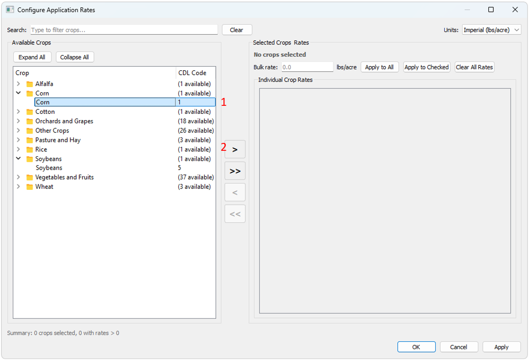
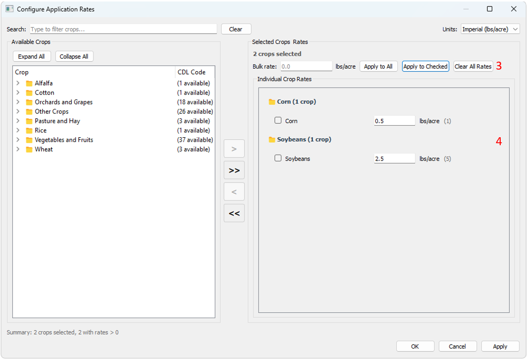
- - Specify the desired units and click "Configure..." to begin configuring crop application rates. For ePest data, only CDL codes related to ePest crop groups with usage data present will be shown.
- Select all crops of interest for a given crop group.
- Click to add selected CDL codes to current crop group, or add all visible CDL codes to current crop group
- Crop application rates may be specified here and applied to all groups or selected groups, or cleared from all groups.
- Crop application rates can also be specified by each CDL code.
- - Specify the offsite transport buffer distance. Distance must be greater than or equal to 0.
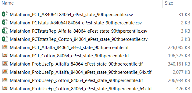
- - Click "Generate Pesticide Use Footprint". APCOAT will generate the following files for each crop in the "\UseFootprints\" folder and be named as shown below:
- A CSV file containing the time series of Percent Crop Treated (PCT) calculations
- [Pesticide]_PCT_[CropApplication Rate]_[Usage Data Source]_[Usage Data Resolution]_[UsageStatistic].csv
- A CSV file containing the statistic calculated from the PCT time series
- [Pesticide]_PCTstatsRep_[Crop]_[Application Rate]_[Usage Data Source]_[Usage Data Resolution]_[UsageStatistic].csv
- A raster showing the PCT values applied for each region
- [Pesticide]_PCT_[Crop]_[ApplicationRate]_[Usage Data Source]_[Usage Data Resolution]_[UsageStatistic].tif
- Probabilistic crop usage footprints.
- [Pesticide]_ProbUseFP_[Crop]_[ApplicationRate]_[Usage Data Source]_[Regional Resolution]_[UsageStatistic].tif
- Downsampled versions of the crop usage footprints for display and review are also created during co-occurrence processing:
- [Pesticide]_ProbUseFP_[Crop]_[ApplicationRate]_[Usage Data Source]_[Usage Data Resolution]_[UsageStatistic]_[2-128]x.tif
|
|
Preparing Custom Usage Data
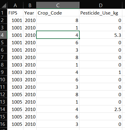
If you wish to load pesticide use data it must be formatted as a comma-separated values (CSV) file conforming to the following requirements.
Templates for county, CRD, and state level pesticide use data files are available and installed by default in "C:\Program Files (x86)\APCOAT\UserDataTemplates".
| Field Title |
Data Type |
Data Requirements |
"State_FIPS" for state resolution
or
"CRD_STASD" for CRD resolution
or
"FIPS" for county resolution
|
Text |
- County and state FIPS codes must match those published by the US Census Bureau[22].
- Crop Reporting District, or Agricultural Statistics District codes must match those published by the National Agricultural Statistics Service[23].
- A lookup table (tbl_FIPS_CRD) joining each of these code sets is available in each project database.
|
| Year |
Integer |
May be 2012 - 2021. Years outside of this range will be ignored. |
| Crop_Code |
Integer |
Crop codes must conform to the following USGS crop groups:
1 - corn
2 - soybeans
3 - wheat
4 - cotton
6 - rice
8 - alfalfa
|
| Pesticide_Use_kg |
Float |
No blanks, must include 0 for years and regions with no use. |
|
Screenshot of example pesticide use data
|
|
Methods
APCOAT uses Maxent software[4] to determine which environmental variables may limit species distributions through comparison of species location records to spatially coincident environmental data, then locates areas with similar environmental values as the basis for generating a Species Distribution Model (SDM). Specifically, Maxent uses presence-only species records to "minimize the relative entropy between two probability densities (one estimated from the presence data and one, from the landscape) defined in covariate space"[24] and generate probabilistic models. Here the user provides the species location records as a CSV file and APCOAT provides the environmental variables that comprise the covariate space as either raster images for terrestrial species or vector files for aquatic species.
This SDM method is employed iteratively in APCOAT, using predictor variable contribution analysis and removal, to select the best-fit model that uses the fewest predictor variables and minimizes correlation among these predictors[18]. Eighty percent of the species location records are used in the initial model training iterations, and the remaining twenty percent of location records are used for evaluation of the final model. Since the probabilistic models vary slightly with each solution, each model iteration is tested using 5 separate model runs with the same selected input variables.
|
|
|
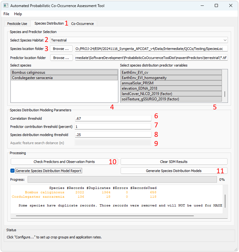
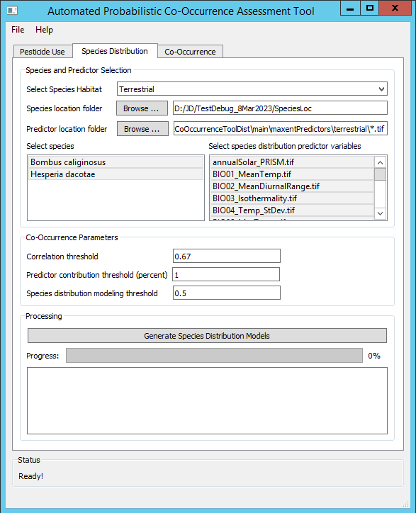
To create probabilistic species distribution models:
- - Click the "Species Distribution" tab.
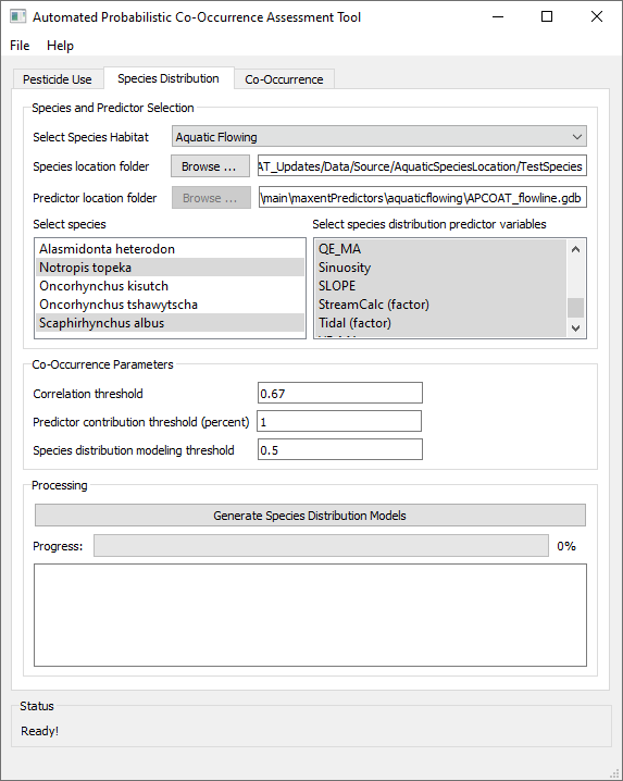
- - Specify the habitat type, "Terrestrial", "Aquatic Flowing", or "Aquatic Static"
- For terrestrial organisms, values of environmental predictor values are joined to each species location record from contiguous raster surfaces covering the continental United States.
- For aquatic organisms, species location records are joined to the nearest flowing waterbody (streams, rivers) or static waterbody (ponds and lakes, limited to waterbodies 0.01 - 10 ha in size) within the distance specified in the "Aquatic feature search distance" input box. If a species record is not within the specified distance of a waterbody the record is excluded from modeling.
Species Selection
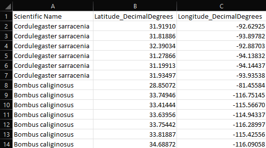
- - Click "Browse ..." and navigate to a folder containing either a single CSV file or multiple CSV files composed of species location data. See below for recommended species location data sources and formatting requirements.
- As the species location data is loaded, APCOAT will perform quality checks to ensure that there are the requisite minimum number of 5 records per species (80% of records are used for model training and 20% for model validation), that there are no formatting errors, and whether or not duplicates exist.
- - Select the species you would like to model which will use the same SDM predictor variables. Hold Ctrl to add single species to the selection, or Shift to add multiple species to the selection.
Environmental Predictor Variable Selection
- - Select the environmental predictor datasets that you would like to evaluate for inclusion in the SDM of the selected species. The available predictor variables for will differ for terrestrial, flowing waterbodies, and static waterbodies. See below for descriptions of the available datasets. By default they will be installed at C:\Program Files (x86)\APCOAT\maxentPredictors. Hold Ctrl to add single variables to the selection, or Shift to add multiple variables to the selection.
-
Whenever possible, take care to select environmental predictor variables that are known to be relevant to the species being modeled, and exclude any variables that may be clearly irrelevant. Here we recommend that predictor variable selection be guided literature review and expert opinion if possible. Whether or not this guidance is available, we recommend a critical review of the final variables that are selected during the automated model iteration and evaluation, as statistical artifacts may persist from bias in species location data collection. For example, results of a SDM may show that a species exhibits a statistical preference for developed areas, when the reality may be that crowd-sourced location data is more likely to come from densely populated areas. In this case, "Frac_Developed" could be excluded from a second round of species distribution modeling.
-
If you are interested in using external environmental predictor variable datasets, they may either be placed in the default predictor folder before project initiation, or selected by clicking "Browse ..." and navigating to a folder containing the SDM predictor variable rasters of interest. See below for formatting requirements for using external rasters and vector datasets.
- If a custom predictor variable is selected that contains categorical data such as land cover, the user must double click the name of the predictor in the selection window and add '(factor)' to the end of the name. This is done automatically for "landCover_NLCD_2019.tif", the land use/land cover raster, and "soilTexture_gSSURGO_2019tif", the soil texture raster, both included with APCOAT.
Model Parameter Selection
- - Specify the correlation threshold. If predictor variables are correlated above this threshold, only the variable with the highest contribution to the distribution model will be kept. All other correlated variables will be excluded.
- - Specify the minimum predictor contribution threshold used to exclude SDM predictor variables.
- - Specify the minimum species distribution modeling threshold. This value is used to filter out low quality habitat values.
- - For aquatic SDMs, specify the aquatic feature search distance.
Modeling Outputs
- - Click "Check Predictors and Observation Points". APCOAT will analyze and report on the alignment of the predictor and observation datasets. For terrestrial SDMs, APCOAT will report if observation points are dropped due to multiple observations being located within the same approximately 800 m pixel, or if observation records are dropped due to being located beyond the extent of a predictor raster and assigned null values for that predictor. For aquatic SDMs, APCOAT will report if observation records are dropped due to being located greater than 100 m from an aquatic feature, or if a selected predictor variable value is null for the closest aquatic feature.
For either type of SDM, the dropped points are compiled for review in tables linked in the species location report.Reviewing these reports can help to decide if the observation points should be retained in modeling by either de-selecting the predictor variable with null values, or editing the location of the record to better align with the predictor variables. If it is determined that the location of the observation records can be reasonably edited to be included in the modeling, the "Clear SDM Results" function must be used before predictor and observation points can be analyzed and reported again.
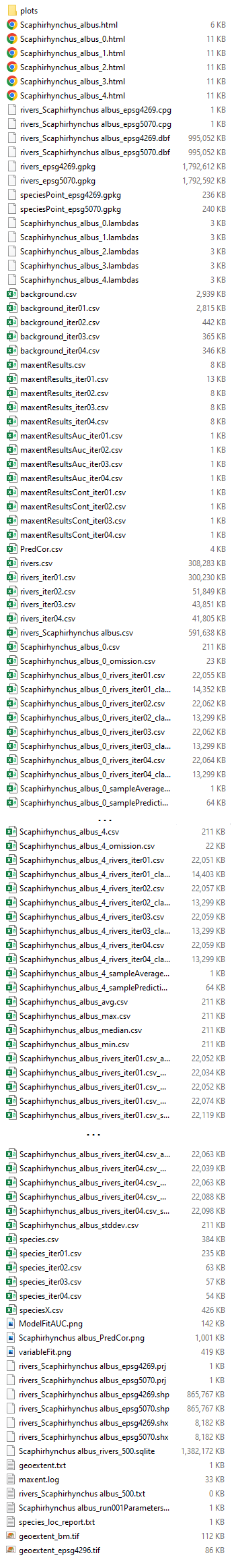
- - Click "Generate Species Distribution Models". APCOAT will generate the following files in the "\SpeciesDistModels\" folder and be named as shown below. If the "Generate Species Distribution Model Report" box is checked, an optional report containing the model inputs and intermediate results will also be generated. Note that especially for terrestrial SDMs the output file sizes can be large for wide-ranging species (> 10 GB):
For terrestrial species
- Final SDM raster without the modeling threshold applied
- [Scientific Name]_sdm_final_raster_raw.tif
- SDM raster showing only values that exceed the modeling threshold
- [Scientific Name]_sdm_final_raster_nan_[threshold].tif
- SDM raster classifying locations where final values exceed the modeling threshold as 1
- [Scientific Name]_sdm_final_raster_msk_[threshold].tif
The following files will also be created when a species is included in a co-occurrence assessment:
- SDM raster rescaled to match the resolution, projection, and cell alignment of the CDL
- [Scientific Name]_sdm_final_raster_nan_[threshold]_res.tif
- Polygon shapefile showing the coverage of the co-occurrence regions where the modeling threshold is exceeded
- [Scientific Name]_[co-occurrence resolution]_[threshold].shp
- Captions for diagnostic image and text files detailing model iteration and production which are included in the assessment report.
For aquatic species
- Shapefile showing the input values used in aquatic features and the statistics of SDM values computed
- rivers_[Scientific Name]_epsg5070.shp
- SDM raster showing only values that exceed the modeling threshold
- [Scientific Name]_sdm_final_raster_nan_[threshold].tif
The following files will also be created when a species is included in a co-occurrence assessment:
- Shapefile showing values of predictor variables analyzed during modeling, and final SDM statistics
- [rivers/ponds]_[Scientific Name]_epsg5070_[threshold].shp
|
Screenshot of example species location file
|
|
Species Location Data
The user may provide their own species occurrence records, or collect them from third parties including:
- FESTF.org - batches of species occurrence records may be accessed through membership.
- GBIF.org - freely available batches of species occurrence records.
- iNaturalist.org - individual species occurrence records, locations of threatened species will be obscured and require additional authorization for access at high resolution.
- NatureServe.org - observation data and Element Occurrence records may be accessed through membership.
When compiling species location data into a single CSV file or multiple CSV files, records must conform to the following requirements:
| Field Title |
Data Type |
Data Requirements |
| Scientific Name |
Text |
|
| Latitude_DecimalDegrees |
Float |
Must be in decimal degrees |
| Longitude_DecimalDegrees |
Float |
Must be in decimal degrees |
A terrestrial and an aquatic example species location dataset[25] are installed by default in C:\Program Files (x86)\APCOAT\SpeciesLocationData\
Species Distribution Predictor Variables
For complete descriptions of all variables see the Environmental Predictor Variable page.
Terrestrial Predictor Variables
The following rasters are included in the APCOAT installation package:
- - Average annual solar radiation, 1990 - 2020[5], annualSolar_PRISM.tif
- - Bioclimatic variables[26] listed in the reference table to the right, derived from 1990 - 2020 climate normals[5], BIO[XX]_[Variable].tif for all 19 variables
- - Distance to saltwater, calculated using NHD flowline and waterbody datasets[7].
- - Distance to freshwater, calculated using NHD flowline and waterbody datasets[7].
- - Elevation[27], elevation_EDNA_2018.tif
- - Land use/land cover[8], landCover_NLCD_2019.tif
- - Soil texture[6], based on representative soil profiles generated by soil series and further simplified to 41 texture classes. soilTexture_gSSURGO_2019.tif
- - Growing season length[8, 9], CHELSA_gsl_1981_2010.tif
- - Köppen climate classification[8, 9], CHELSA_kg0_1981-2010.tif
- - Net primary productivity[8, 9], CHELSA_npp_1981-2010.tif
- - Potential evapotranspiration during wettest/driest/warmest/coldest quarters[8, 9], CHELSA_pet_MaxPrecipQuarter.tif
- - Site water balance[8, 9], CHELSA_swb_2018.tif
- - Habitat heterogeneity[10], EarthEnv_EVI_cv.tif
Aquatic Predictor Variables
The following fields and data for SDM of flowing waterbodies are included in the APCOAT installation package:
- - BIO[XX]_[Variable], the mean value within the flowline catchment for all 19 BioClim variables
- - FCODE, the flowline type
- - Frac_[Class], the fraction of the given land use/land cover class found within a 100m buffer of the flowline[8]
- - MAXELEVSMO, elevation in meters[7]
- - StreamCalc, order of stream [7]
- - Tidal, 1 indicates the waterbody is tidal, 0 indicates that it is not[7]
- - SLOPE, [7]
- - Sinuosity, calculated as sinuousity = [flowline length]/[distance between flowline endpoints]
- - QE_MA, mean annual flow rate[7]
- - QE_StDev, standard deviation of monthly flow rates[7]
- - *VE_MA, mean annual velocity[7]. *Note that tidal flowlines and those impounded by dams are assigned a dummy value of 0.001 so this variable is not recommended for use for species found in those areas.
- - VE_StDev, standard deviation of monthly velocity[7]
- - D50_mm_, median bed-material particle size[28]
- - Selected StreamCat variables, described in the Environmental Predictor Variable page
The following fields and data for SDM of static waterbodies are included in the APCOAT installation package:
- - Area_sq_km, area of the waterbody in square kilometers[7]
- - BIO[XX]_[Variable], the mean value within the waterbody for all 19 BioClim variables
- - Elevation_m, minimum elevation detected within the waterbody [27]
- - FCODE, waterbody type[7]
- - Frac_[Class], the fraction of the given land use/land cover class found within a 100m buffer of the waterbody[8]
- - Length_div_Area, the ratio of the waterbody perimeter to area
- - ONOFFNET, 1 indicates that the waterbody is hydrologically connected to flowing waterbodies, 0 indicate that it is not[7]
- - Selected LakeCat variables, described in the Environmental Predictor Variable page
Using Additional Predictor Variables
Rasters used in APCOAT species distribution modeling must be of identical resolution, projection, extent, and cell alignment. As such, in order to use additional predictor variable rasters the user may need to modify either the additional rasters or the existing ones if they are to be used together. Additional rasters can also be used independently of the rasters provided with APCOAT. Resampling, reprojection, and cell alignment functions are available in GIS software such as ArcGIS or QGIS. The bioclimatic, land cover, soil texture, elevation, and solar radiation raster datasets provided with APCOAT for terrestrial species distribution modeling are of 5 arc minute spatial resolution (approximately 800 m) and projected using the GCS_North_American_1983 projection, WKID: 4269.
At this time, APCOAT does not support the use of additional vector predictor datasets. However, additional data may be appended to the existing flowline and waterbody datasets using GIS software. Since Maxent evaluates all possible features within the species range, any null values present in the additional data will result in an erroneous model where habitat quality predictions cannot be properly matched to spatial features.
Reference table for Flowing Aquatic FCODEs
| FCODE | Description |
|---|
| 33400 | Connector (no attributes) |
| 33600 | CanalDitch (CanalDitch Type = null) |
| 33601 | CanalDitch (CanalDitch Type = Aqueduct) |
| 33603 | CanalDitch (CanalDitch Type = Stormwater) |
| 42800:42823 | Pipelines |
| 46000 | StreamRiver (no attributes) |
| 46003 | StreamRiver (Hydrographic Category = Intermittent) |
| 46006 | StreamRiver (Hydrographic Category = Perennial) |
| 46007 | StreamRiver (Hydrographic Category = Ephemeral) |
| 55800 | Artificial Path (no attributes) - Note that many of these have been filtered out from the NHDPlus database since they are either represented by waterbodies, or modeled predictor values are unavailable or unreliable. This may cause some flowline SDMs to not appear as fully connected hydrologic networks. |
|
Reference table for Land Use/Land Cover Values derived from NLCD 2019
1 - water
2 - developed
3 - barren
4 - forest
5 - shrub/herb
6 - pasture/hay
7 - cultivated
8 - wetland
|
Reference table for WorldClim bioclimatic variables
BIO1 = Annual Mean Temperature
BIO2 = Mean Diurnal Range (Mean of monthly (max temp - min temp))
BIO3 = Isothermality ((BIO2/BIO7) x100)
BIO4 = Temperature Seasonality (standard deviation x100)
BIO5 = Max Temperature of Warmest Month
BIO6 = Min Temperature of Coldest Month
BIO7 = Temperature Annual Range (BIO5-BIO6)
BIO8 = Mean Temperature of Wettest Quarter
BIO9 = Mean Temperature of Driest Quarter
BIO10 = Mean Temperature of Warmest Quarter
BIO11 = Mean Temperature of Coldest Quarter
BIO12 = Annual Precipitation
BIO13 = Precipitation of Wettest Month
BIO14 = Precipitation of Driest Month
BIO15 = Precipitation Seasonality (Coefficient of Variation)
BIO16 = Precipitation of Wettest Quarter
BIO17 = Precipitation of Driest Quarter
BIO18 = Precipitation of Warmest Quarter
BIO19 = Precipitation of Coldest Quarter
|
Reference table for gSSURGO Soil Texture variables
| Value | Texture |
|---|
| 1 | Artifacts |
| 2 | Coarse sand |
| 3 | Loam |
| 4 | Clay loam |
| 5 | Coarse sandy loam |
| 6 | Fine sandy loam |
| 7 | Silt loam |
| 8 | Sandy loam |
| 9 | Loamy fine sand |
| 10 | Loamy sand |
| 11 | Loamy very fine sand |
| 12 | Sand |
| 13 | Silty clay |
| 14 | Silty clay loam |
| 15 | Very fine sandy loam |
| 16 | Bedrock |
| 17 | Boulders |
| 18 | Clay |
| 19 | Loamy coarse sand |
| 20 | Slightly decomposed plant material |
| 21 | Fine sand |
| 22 | Cobbles |
| 23 | Very fine sand |
| 24 | Highly decomposed plant material |
| 25 | Moderately decomposed plant material |
| 26 | Peat |
| 27 | Sandy clay loam |
| 28 | Muck |
| 29 | Material |
| 30 | Cinders |
| 31 | Consolidated permafrost |
| 32 | Fine gypsum material |
| 33 | Fragmental material |
| 34 | Gravel |
| 35 | Silt |
| 36 | Gypsiferous material |
| 38 | 0 |
| 39 | Sandy clay |
| 40 | Stones |
| 41 | Unweathered bedrock |
| 42 | Variable |
| 43 | Water |
Reference table for Static Aquatic FCODEs
| FCODE | Description |
|---|
| 36100 | Playa |
| 39000 | Lake/Pond - feature type only: no attributes |
| 39001 | Lake/Pond - Hydrographic Category|intermittent |
| 39004 | Lake/Pond - Hydrographic Category|perennial |
| 39005 | Lake/Pond - Hydrographic Category|intermittent; Stage|high water elevation |
| 39006 | Lake/Pond - Hydrographic Category|intermittent; Stage|date of photography |
| 39009 | Lake/Pond - Hydrographic Category|perennial; Stage|average water elevation |
| 39010 | Lake/Pond - Hydrographic Category|perennial; Stage|normal pool |
| 40307 | Inundation |
| 43600:43624 | Reservoirs |
| 46600 | SwampMarsh (Hydrographic Category = null) |
| 49300 | Estuary (no attributes) |
|
|
Methods
With APCOAT, co-occurrence for terrestrial species is measured by multiplying batches of SDM rasters by pesticide use footprints and summarizing the resulting rasters by zones of interest for ease of interpretation. When calculating co-occurrence APCOAT will also produce a report detailing the inputs variables, methods, and outputs involved in each step of the analysis.
For co-occurrence assessments of aquatic species, the probabilities of co-occurrence are calculated differently for flowing and static waterbodies (Figure 2). High resolution drainage areas (2,647,454 features within the CONUS at 1:24,000 scale[7]) are used to calculate the probability that terrestrial pesticide applications will be transported to flowing aquatic environments such as streams and rivers. The methods used to calculate the probability of pesticide transport are distinct for segments that receive flow from neighboring HUC12 watersheds (mainstems) and those that do not (tributaries). Mainstems are defined as flowlines with an associated drainage area[7] that is greater than the drainage area of the HUC12 they are situated within. For mainstems, the mean and maximum values of the usage footprint within the associated local HUC12 watershed are calculated, as well as the mean and maximum values of all upstream HUC12 watersheds combined. For tributaries, the mean and maximum values of the usage footprint are calculated within the associated local catchment, as well as the same values for all upstream catchments combined. The set of transport probabilities that is most appropriate for a given chemical will be dependent on its persistence and mobility. The pesticide presence probabilities based on local usage would be most relevant for quickly degrading pesticides, or pesticides with drift-dominated transport to aquatic systems. The pesticide presence probabilities based on upstream usage would be most relevant for persistent pesticides, or pesticides with runoff-dominated transport to aquatic systems.
Polygon shapefiles may be loaded to represent species locations deterministically. These may be areas such as species ranges, critical habitat, known locations, or Pesticide Use Limitation Areas (PULAs) where pesticide co-occurrence is of interest.
|

|
|
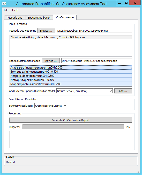
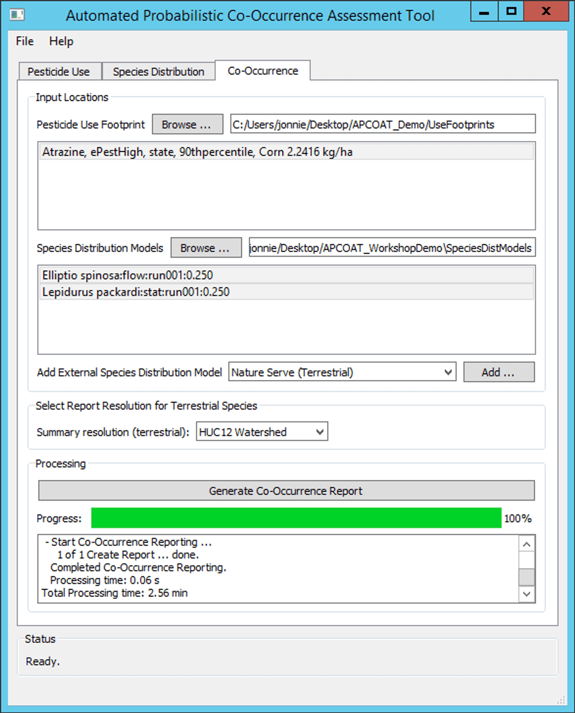
To create probabilistic co-occurrence assesments:
- - Click the "Co-Occurrence" tab.
- - Confirm that the path to the use footprints folder is correctly associated with the current project. If not, click "Browse..." and navigate to the "UseFootprints" folder associated with the currently loaded assessment project database.
- - Select the crop footprints of interest.
- - Confirm that the path to the SDM folder is correctly associated with the current project. If not, click "Browse..." and navigate to the "SpeciesDistModels" folder associated with the currently loaded assessment project database.
- - Select the SDMs of interest.
- - (Optional). Select external NatureServe SDMs of interest.
a - Provide a species name for the external SDM.
b - Specify the path of the .TIF file of the external SDM.
c - Specify the desired SDM threshold. Values below this threshold will be excluded from co-occurrence modeling.
d - Include helpful metadata for the external SDM that will be included in the co-occurrence report.
e - Click Submit to apply the modeling threshold and load the external SDM into the database.
- - (Optional). Add Pesticide Use Limitation Areas (PULA) polygons of interest.
a - Provide a name for the external PULA.
b - Specify the PULA type (Terrestrial, Aquatic Flowing, Aquatic Static).
c - Specify the path of the external .SHP and associated files for the PULA of interest.
d - Include helpful metadata for the external SDM that will be included in the co-occurrence report.
e - Click Submit to load the external PULA into the database.
- - Select the desired summary resolution.
- - Click "Generate Co-Occurrence Report". APCOAT will generate the following files for each combination of crop and species analyzed in "[Project Folder]\CoOccurrence\[Usage Footprint]\[Species name]\[SDM run number]\..." and be named as shown below:
|

|
| Inputs
- The desired output is the probabilistic usage of malathion on alfalfa and cotton.
- The usage data statistic of interest is the 90th percentile of annual usage as measured by USGS ePest estimates.
- Application rates are provided in imperial units, 7.5 lbs/acre for both alfalfa and cotton.
- Processing time was 70 minutes using a laptop with an Intel(R) Core(TM) i7-7500U CPU @ 2.70GHz processor and 8 GB of RAM.
|
 |
Intermediate Results
* indicates data will be included in co-occurrence report
- Malathion_PCT_A84064T84064_ePest_state_90thpercentile.csv
- Pesticide usage, maximum potential usage, and PCT for all crops, years, and regions
- Malathion_PCTstats_A84064T84064_ePest_state_90thpercentile.csv
- The annual usage statistic (90th percentile) calculated for each crop and region
- * Malathion_PCTstatsRep_Alfalfa_84064_ePest_state_90thpercentile.csv
- A range of statistics from minimum to maximum for a single crop and each region
- Malathion_PCT_Alfalfa_84064_ePest_state_90thpercentile.tif
- The national PCT raster generated for the specified usage statistic and crop at 30m resolution. The raster is in integer format and multiplied by a factor of 10,000 such that 100% PCT = 10,000 and 50% PCT = 5,000.
- Malathion_ProbUseFp_Alfalfa_84064_ePest_state_90thpercentile.tif
- The national probabilistic usage raster for the specified usage statistic and crop at 30m resolution. The raster is in integer format and multiplied by a factor of 10,000 such that 100% usage probability = 10,000 and 50% usage probability = 5,000. It is produced by multiplying the PCT raster by the probabilistic crop footprint included in the APCOAT installation.
- Malathion_ProbUseFp_Alfalfa_84064_ePest_state_90thpercentile_64x.tif
- The national probabilistic usage raster for the specified usage statistic and crop, showing the maximum values from the above raster at 1/64th the original spatial resolution (1,920m). The raster is in integer format and multiplied by a factor of 10,000 such that 100% usage probability = 10,000 and 50% usage probability = 5,000.
|
|
|
Co-Occurrence Report Result
When a given probabilistic crop footprint is selected for use in a co-occurrence report, the map figure shown here will be automatically generated and included in the report document and co-occurrence folder ([Project Folder]\CoOccurrence\Malathion_ProbUseFp_Alfalfa_84064_ePest_state_90thpercentile.png). This example is for the 90th percentile of annual malathion usage by state as measured by USGS ePest estimates, multiplied by the probability that a given 30m pixel will be planted with alfalfa as measured by the USDA Cropland Data Layer.
|
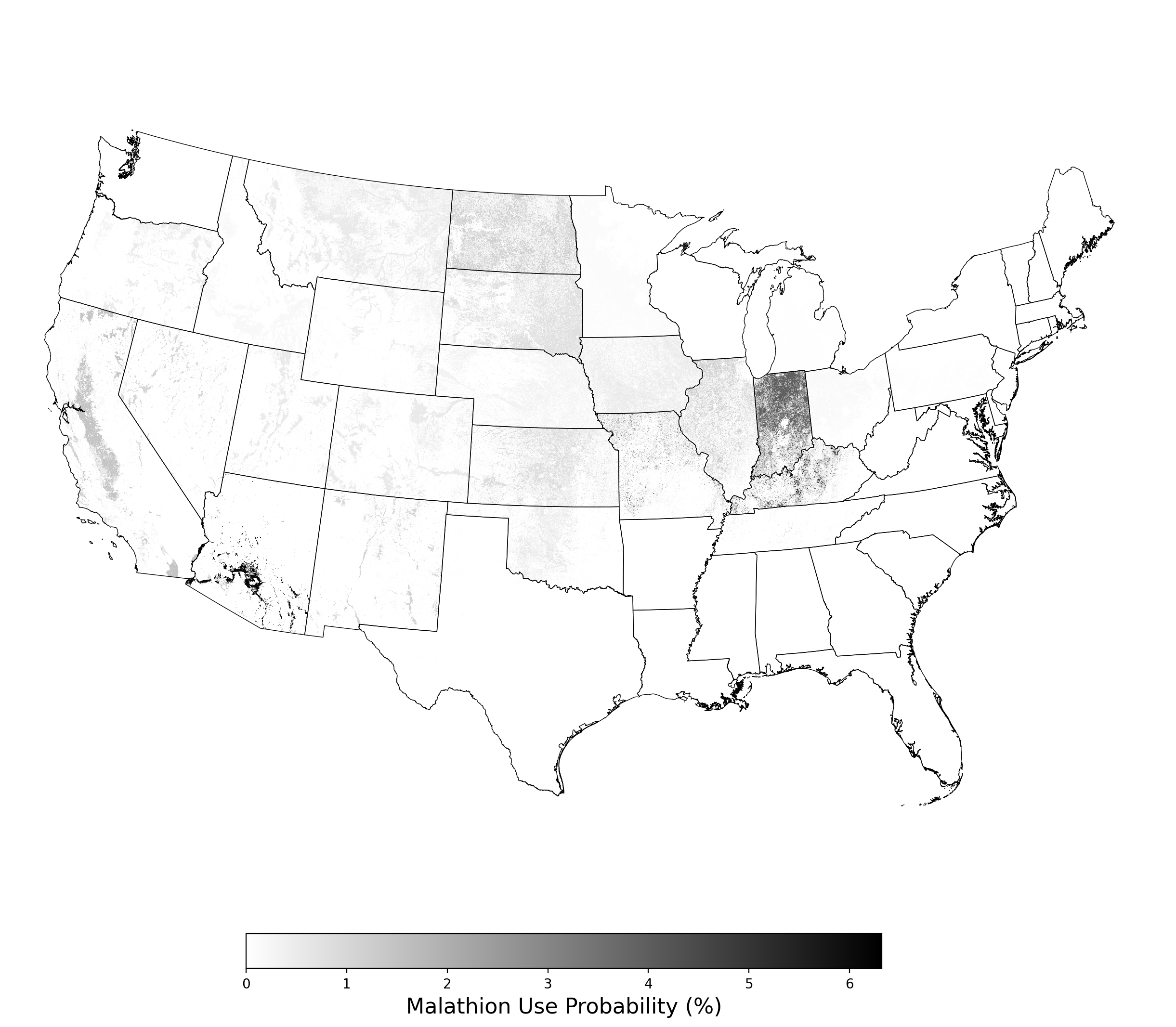
Figure 1. Probabilistic use footprint for malathion applications on alfalfa. |
Inputs
- The desired outputs are Species Distribution Models (SDM) for two species, Bombus caliginosus and Hesperia dacotae.
- The selected species distribution predictor variables include all of the terrestrial predictor variables included with APCOAT.
- The correlation threshold used to exclude combinations of predictors that are strongly correlated with one another is left at the default value of 0.67.
- The predictor contribution threshold used to exclude predictors during iterative model evaluation is left at the default value of 1 percent.
- The species distribution modeling threshold used to filter out regions of low quality habitat is specified at 0.5. Regions of the final SDM with probabilistic habitat quality below 50% will not be included in the output raster.
- Processing time was 80 minutes using a laptop with an Intel(R) Core(TM) i7-7500U CPU @ 2.70GHz processor and 8 GB of RAM.
|
 |
Intermediate Results
* indicates data will be included in co-occurrence report
- *Bombus caliginosus_run001Parameters.txt
- Each modeling parameter is listed on a separate line: all species predictor variable file names, discrete predictor variable file names, predictor correlation threshold, predictor contribution threshold
- *Bombus caliginosus_PredCor.png
- Correlation between predictor variables
- Bombus caliginosus_sdm_iter[1...5]_real[1-5].rds
- Intermediate modeling SDM results. Five model realizations are generated for each iteration of predictor variable combinations. In this example five iterations were run before iteration number 4 was chosen.
- Bombus caliginosus_Contribution_Iter[1-X]_Real[1-5].png
- The contribution of each predictor variable for all 5 realizations of each model iteration.
- Bombus caliginosus_ResTable_Iter[1-5].rds
- Diagnostic statistics for all 5 realizations of each model iteration.
- Bombus caliginosus_ResVarsTable_Iter[1-5].rds
- Table showing the contribution of each predictor variable for all 5 realizations of each iteration.
- *Bombus caliginosus_ModelFitAUC_iter[3-5].png
- Model fit as measured by total Area Under Curve for each model iteration and all previous iterations.
- Bombus caliginosus_sdm_final_iter4_real[1-5].rds
- Five realizations of the final selected SDM iteration.
- Bombus caliginosus_sdm_final_raster.png
- A map showing the average of the five final SDM realizations, and species locations. Be sure to consider any restrictions associated with redistributing species location data when publishing this figure.
- Bombus caliginosus_sdm_sd_final_raster.png
- A map showing the standard deviation of the five final SDM realizations, and species locations. Be sure to consider any restrictions associated with redistributing species location data when publishing this figure.
- Bombus caliginosus_sdm_final_raster_raw.tif
- The final SDM raster without the species distribution model threshold applied.
- *Bombus caliginosus_final_stats.csv
- CSV version of ResTable_Iter[1-5] for the final selected model iteration.
- *Bombus caliginosus_sdm_final_auc.csv
- Model fit as measured by Area Under Curve for each of the five realizations of the final model iteration.
- *Bombus caliginosus_sdm_final_contribution.png
- Contribution to model of each predictor variable included in the final model iteration.
- *Bombus caliginosus_sdm_final_contvariablefit.png
- The distributions of values sampled randomly and from species observations for all continuous variables included in the final model iteration. Since these graphs are produced via kernel density estimation, the initial estimated ranges may extend beyond the true range of the variables (e.g. fractions of land greater than 100 or less than 0). In these cases the ranges are truncated and density is set to 0 outside the true variable range..
- *Bombus caliginosus_sdm_final_discvariablefit.png
- The distributions of values sampled randomly and from species observations for all discrete variables included in the final model iteration.
- Bombus caliginosus_sdm_final_raster_zer_500.tif
- A raster of the final model iteration with the species distribution model threshold applied. Values below the threshold are set to 0.
- Bombus caliginosus_sdm_final_raster_nan_res_ext_500.tif
- The raster described above, resampled and reprojected to match the projection, resolution, and alignment of APCOAT pesticide usage footprints.
- Bombus caliginosus_sdm_sd_final_raster.tif
- A raster showing the standard deviation of the five realizations of the final model iteration.
- Bombus caliginosus__[County, CRD, HUC8, HUC12, State]_[threshold].shp (and associated .dbf, .prj, .shx files)
- The zones of interest within the extent of the final model iteration. These are generated when a species is selected for inclusion in a co-occurrence report.
|
 |
| Co-Occurrence Report Result
When a given species crop footprint is selected for use in a co-occurrence report, the map figure shown here will be automatically generated and included in the report document and co-occurrence folder ([Project Folder]\CoOccurrence\HabitatSuitability_200.png). This example is for Bombus caliginosus, modeled with all of the recommended bioclimatic and elevation predictors, as well as the land use/land cover predictor included with APCOAT, and a model threshold of 50%.
|
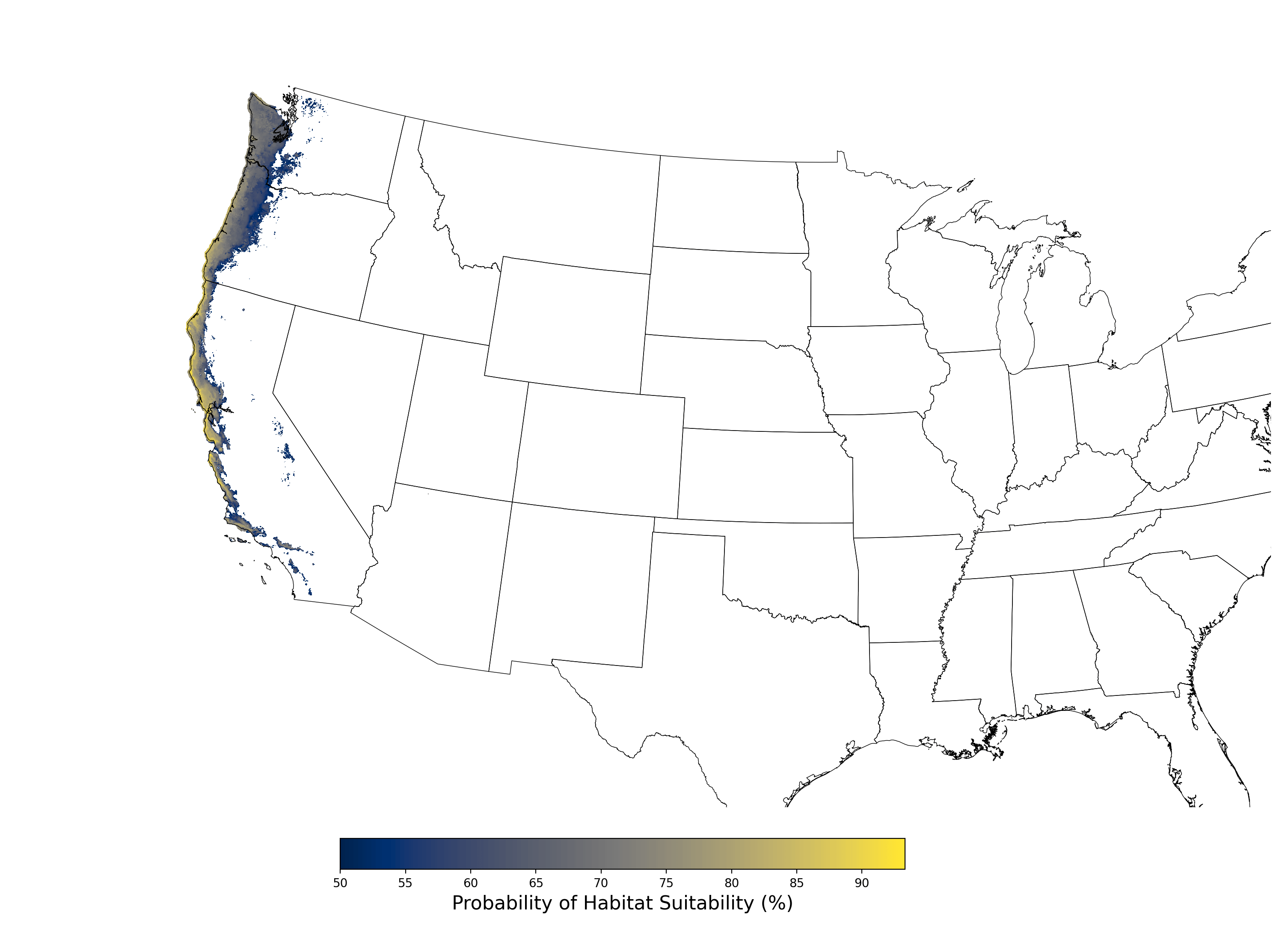
Figure 8. Final mean SDM output for Bombus caliginosus. |
Inputs
- The desired outputs are Species Distribution Models (SDM) for two species, Notropis topeka and Scaphirhynchus albus.
- The selected species distribution predictor variables include all of the static aquatic predictor variables included with APCOAT.
- The correlation threshold used to exclude combinations of predictors that are strongly correlated with one another is left at the default value of 0.67.
- The predictor contribution threshold used to exclude predictors during iterative model evaluation is left at the default value of 1 percent.
- The species distribution modeling threshold used to filter out regions of low quality habitat is specified at 0.5. Regions of the final SDM with probabilistic habitat quality below 50% will not be included in the output raster.
- Processing time was 60 minutes using a laptop with an Intel(R) Core(TM) i7-7500U CPU @ 2.70GHz processor and 8 GB of RAM.
|
 |
Intermediate Results
* indicates data will be included in co-occurrence report
- Scaphirhynchus_albus.html
- A summary of the five model realizations conducted (i.e. Scaphyrhynchus_albus_0.html - Scaphyrhynchus_albus_4.html) using Maxent. Includes analyses of omission/commission, response curves selected for each predictor variable, and variable contributions.
- rivers_epsg[4269/5070].gpkg
- GeoPackage file showing predictor values of flowlines used within species modeling extent.
- speciesPoint_epsg[4269/5070].gpkg
- GeoPackage file showing the species location records used in modeling.
- background_iter[XX].csv
- Values collected during background sampling.
- *maxentResults_iter[XX].csv
- Iterative statistical evaluation of Maxent modeling results.
- Scaphirhynchus_albus_[0-4]*.csv.gpkg
- Intermediate Maxent processing files.
- *ModelFitAUC.png
- Model fit as measured by total Area Under Curve for each model iteration.
- *Scaphirhynchus_albus_PredCor.png
- Correlation between predictor variables at species locations.
- *variableFit.png
- Graphs comparing predictor variable values at species locations and randomly sited background samples. Since these graphs are produced via kernel density estimation, the initial estimated ranges may extend beyond the true range of the variables (e.g. fractions of land greater than 100 or less than 0). In these cases the ranges are truncated and density is set to 0 outside the true variable range.
- rivers_Scaphirhynchus albus_epsg[4269,5070].shp
- Shapefile showing flowlines, their predictor values, their final SDM values.
- *geoextent_bm.tif
- Image showing the spatial extent of the SDM.
|
 |
| Co-Occurrence Report Result
When a given species is selected for use in a co-occurrence report, the map figure shown here will be automatically generated and included in the report document and co-occurrence folder (run[XXX]_[speciesThreshold]\[rivers/ponds]_coo_[summaryResolution]_[Species name]__epsg5070.png). This example is for Scaphirhynchus albus, modeled using aquatic flowing predictors included with APCOAT, and a model suitability threshold of 50%.
|
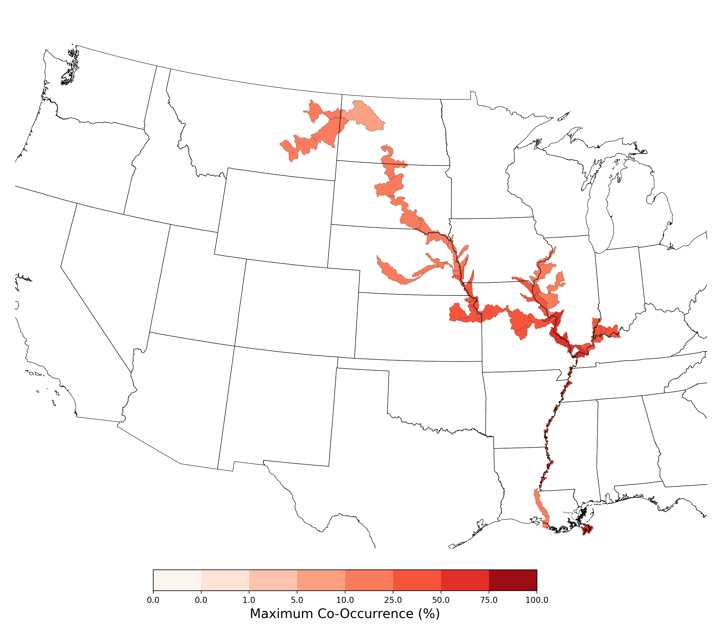
Figure 8. Final mean SDM output for Scaphirhynchus albus. |
| Inputs
- The desired outputs are reports on probabilistic spatial co-occurrence between applications of atrazine to corn, and areas where the probability of suitable habitat is greater than 50% for three terrestrial species: Arabis serotina (imported from a NatureServe SDM), Bombus caliginosus and Hesperia dacotae, and two aquatic species: Notropis topeka and Scaphirhynchus albus.
- The spatial co-occurrence is to be summarized by Crop Reporting District for visualization purposes.
- Processing time was 36 minutes using a laptop with an Intel(R) Core(TM) i7-7500U CPU @ 2.70GHz processor and 8 GB of RAM.
|
 |
Intermediate Results
* indicates data will be included in co-occurrence report
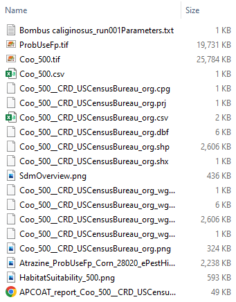
- \[Project Folder]\CoOccurrence\Atrazine\Corn_28020_ePestHigh_state_Maximum\Bombus caliginosus\run001_500
- Directory for results of a single co-occurrence assessment. Separate directories are created for each combination of species and crop.
- *Bombus caliginosus_run001Parameters.txt
- A copy of the SDM input parameters file. Each modeling parameters is listed on a separate line: all species predictor variable file names, discrete predictor variable file names, predictor correlation threshold, predictor contribution threshold.
- ProbUseFp.tif
- Probabilistic use footprint raster clipped to the extent of the species distribution model. The raster is in integer format and multiplied by a factor of 10,000 such that 100% usage probability = 10,000 and 50% usage probability = 5,000.
- Coo_500.tif
- Raster showing values of probabilistic co-occurrence between pesticide usage raster and SDM raster at 30m resolution
- *Coo_500.csv
- Table showing min, mean, and max values of probabilistic co-occurrence between pesticide usage raster and SDM raster at summary zone resolution
- *Coo_500__CRD_USCensusBureau_org.csv
- Zonal summary of average co-occurrence raster values
- Coo_500__CRD_USCensusBureau_org.shp (and associated .dbf, .prj, .shx files)
- Shapefile containing zonal averages of co-occurrence raster values
- * SdmOverview.png
- Map of the extent of the SDM
- Coo_500__CRD_USCensusBureau_org_wgs84.shp (and associated .dbf, .prj, .shx files)
- Shapefile containing zonal averages of co-occurrence raster values, projected to the WGS 1984 datum
- *Coo_500__CRD_USCensusBureau_org.png
- Map of zonal co-occurrence averages
- *Atrazine_ProbUseFp_Corn_28020_ePestHigh_state_Maximum.png
- Map of pesticide usage probability
- *HabitatSuitability_500.png
- Map of habitat suitability derived from SDM
- APCOAT_report_Coo_500__CRD_USCensusBureau_org.html
- Probabilistic co-occurrence report containing modeling inputs, outputs, and assessment
|
 |
| Co-Occurrence Report Results
A report containing model inputs and outputs will be generated for each selected combination of species and crop and located in
\[Project Folder]\CoOccurrence\[Pesticide]\[Crop]_[Application Rate]_[Usage Data Source]_[Usage Data Summary Resolution]_[Usage Data Statistic]\[Species]\[SDM Version_Threshold]\.
The example table shows statistics regarding co-occurrence over the species range. The example figure shows probabilistic co-occurrence between the extent of the SDM of Bombus caliginosus and atrazine applications on corn, summarized at the CRD scale. An example case study composed of ten compiled co-occurrence reports is available at https://stone-env.com/APCOAT.
|
Table 6. Statistics of probabilistic co-occurrence between the range of Bombus caliginosus and atrazine applications on cotton.
| Number of CRD polygons included in assessment |
18 |
| Maximum of maximum co-occurrence by CRD |
1.79e+01% |
| Minimum of maximum co-occurrence by CRD |
0.00e+00% |
| Average co-occurrence for species range |
1.24e-02% |
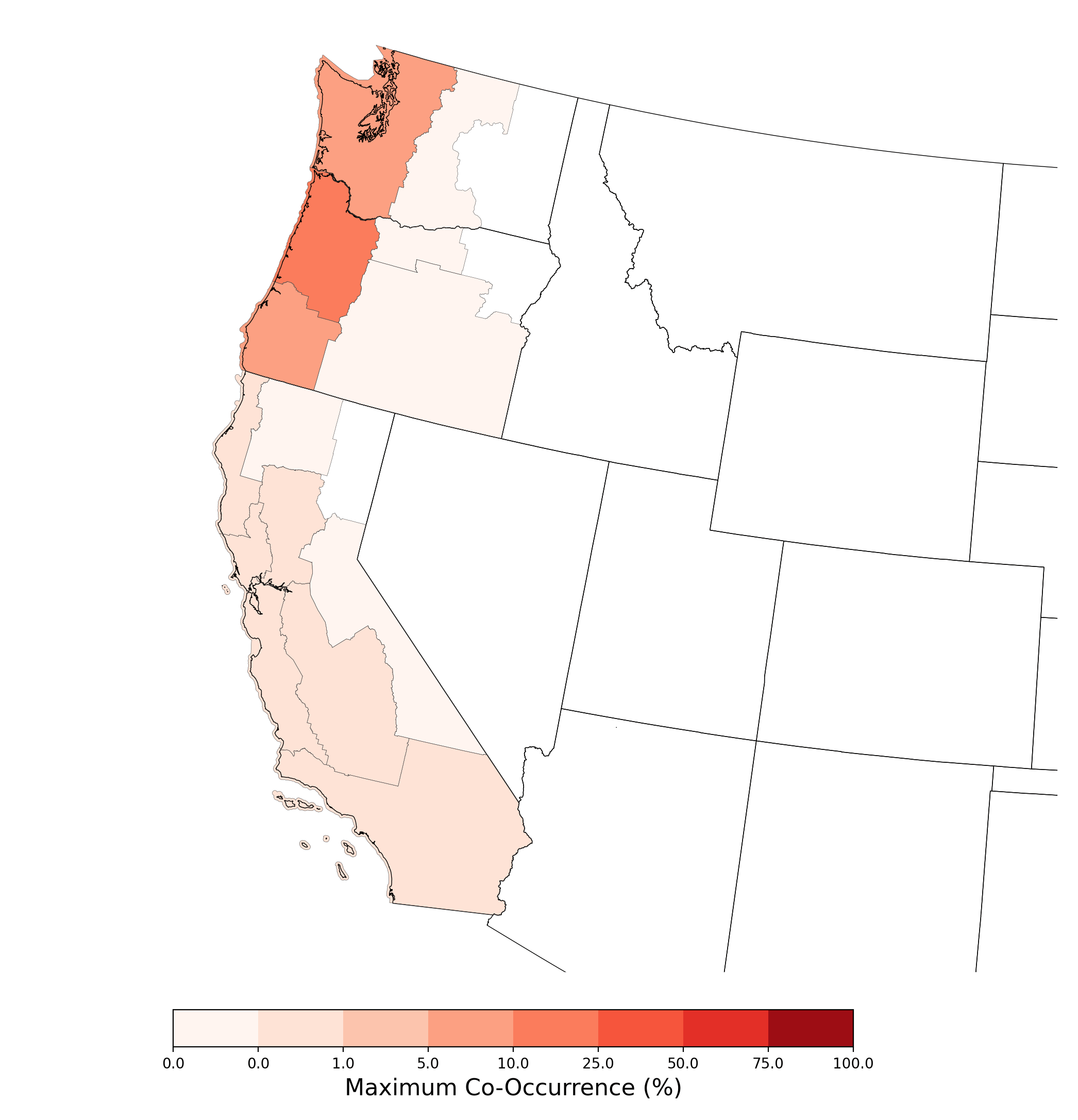
Figure 9. Map showing probabilistic co-occurrence between the range of Bombus caliginosus and atrazine applications on corn, summarized at the CRD scale. |
| Inputs
- The desired outputs are reports on probabilistic spatial co-occurrence between applications of atrazine to corn, and areas where the probability of suitable habitat is greater than 25% for two aquatic species: Elliptio spinosa and Lepidurus packardi.
- The spatial co-occurrence is to be summarized by HUC12 for visualization purposes.
- Processing time was 24 minutes using a laptop with an Intel(R) Core(TM) i7-7500U CPU @ 2.70GHz processor and 8 GB of RAM.
|
 |
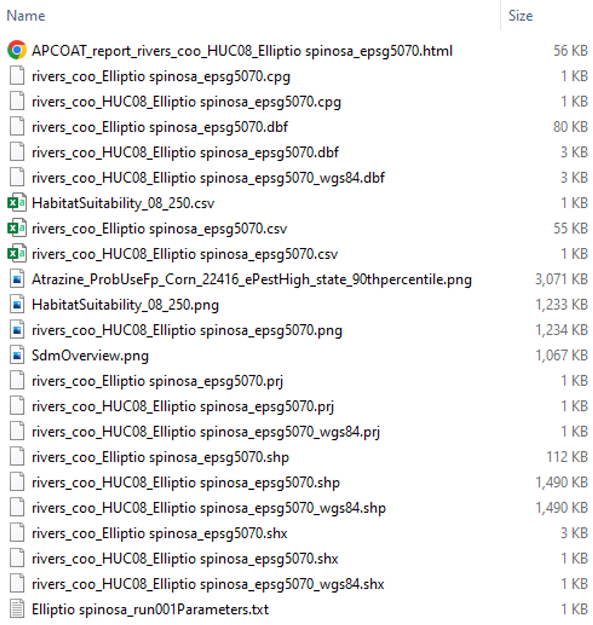
Intermediate Results
The intermediate results for an aquatic co-occurrence analysis are similar to those for a terrestrial analysis. The primary difference is that the results of the SDM process and co-occurrence calculations are stored in vector format (lines for flowing aquatic habitats, polygons for static aquatic habitats). The example shown to the right is for a static aquatic analysis, for flowing aquatic analyses the resulting files will be similar, with "rivers" in place of "ponds" in the filenames.
Co-occurrence results at the flow line or pond level are found in the following fields in the [ponds/rivers]_coo_[species]_epsg5070.shp files:
- comid: Feature identifier
- avg_habsui: Average habitat suitability
- local_mean: Local mean usage probability
- local_max_: Local maximum usage probability
- upstream_m: Upstream mean usage probability
- upstream_1: Upstream max usage probability
- local_me_1: Local mean co-occurrence
- local_ma_1: Local max co-occurrence
- upstream_2: Upstream mean co-occurrence
- upstream_3: Upstream max co-occurrence
The maximum values of the pond or river features are aggregated to the selected summary region in the following fields in the [ponds/rivers]_coo_[region]_[species]_epsg5070.shp files:
- nmb_lines/ponds: Number of lines considered within region (i.e., number of suitable habitat flow lines)
- max_avg_ha: Maximum habitat suitability index
- max_local_: Maximum of local mean usage probability
- max_loca_1: Maximum of local maximum usage probability
- max_upstre: Maximum of upstream mean usage probability
- max_upst_1: Maximum of upstream maximum usage probability
- max_loca_2: Maximum of local mean co-occurrence
- max_loca_3: Maximum of local maximum co-occurrence
- max_upst_2: Maximum of upstream mean co-occurrence
- max_upst_3: Maximum of upstream maximum co-occurrence
|
 |
| Co-Occurrence Report Results
A report containing model inputs and outputs will be generated for each selected combination of species and crop and located in
\[Project Folder]\CoOccurrence\[Pesticide]\[Crop]_[Application Rate]_[Usage Data Source]_[Usage Data Summary Resolution]_[Usage Data Statistic]\[Species]\[Habitat Type]\[SDM Version_Threshold]\.
The example table shows statistics regarding co-occurrence over the species range. The example figure shows probabilistic co-occurrence between the extent of the SDM of Elliptio spinosa and atrazine applications on corn, summarized at the HUC8 scale. An example case study composed of ten compiled co-occurrence reports is available at https://stone-env.com/APCOAT.
|
Table 7. Statistics of probabilistic co-occurrence between the range of Elliptio spinosa and atrazine applications on cotton.
| Number of HUC08 polygons included in assessment |
11 |
| Maximum average HUC08 co-occurrence |
8.07e+01% |
| Minimum average HUC08 co-occurrence |
1.92e+01% |
| Local co-occurrence using mean pesticide usage |
4.08e-01% |
| Local co-occurrence using maximum pesticide usage |
3.49e+01% |
| Upstream co-occurrence using mean pesticide usage |
2.52e-01% |
| Upstream co-occurrence using maximum pesticide usage |
4.50e+01% |
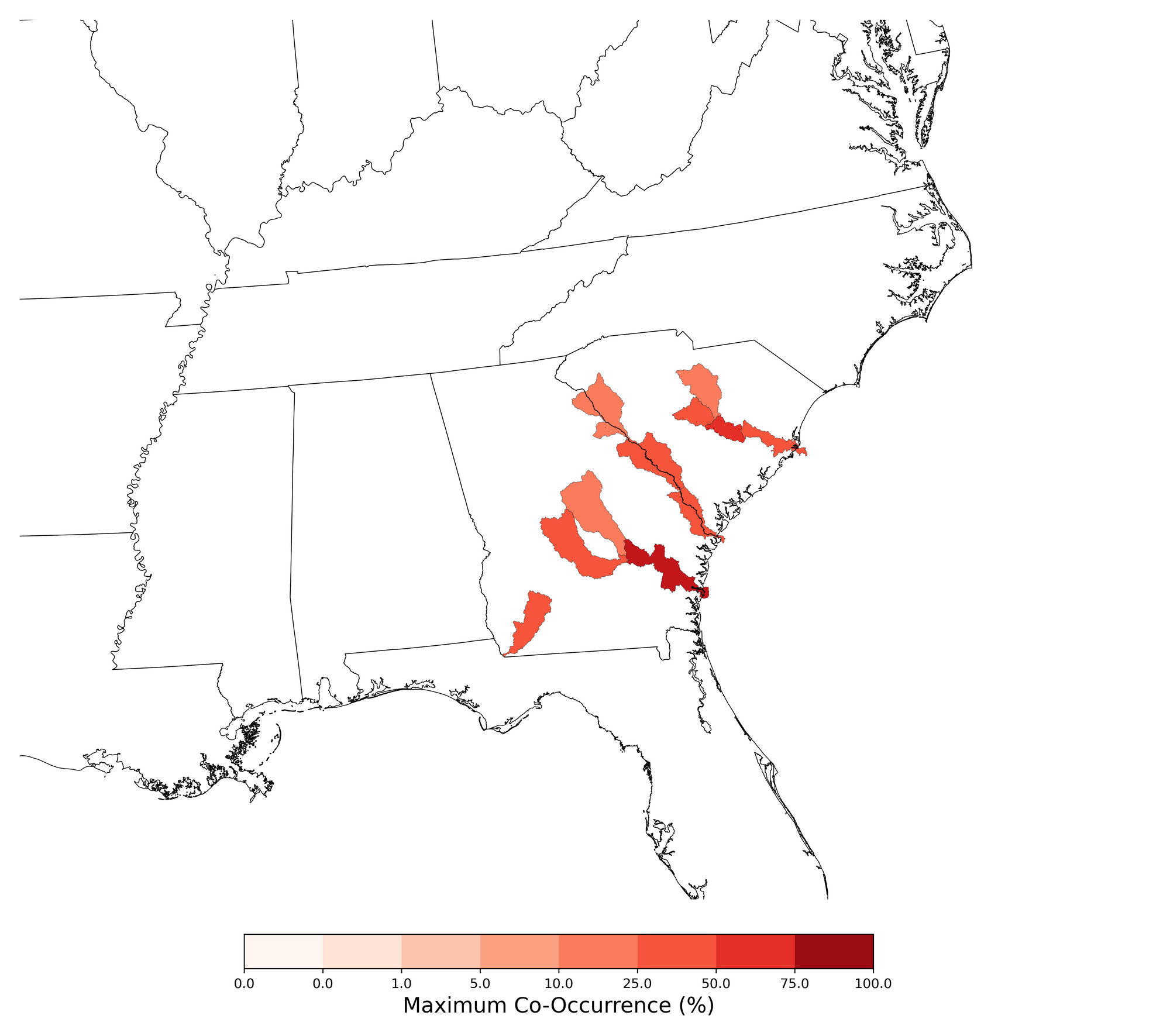
Figure 10. Map showing probabilistic co-occurrence between the range of Elliptio spinosa and atrazine applications on corn, summarized at the HUC8 scale. |
